Homogenization schemes

Before this page

Concentration and contribution tensors, where the dilute concentration tensor and the contribution tensors and are defined, Crack opening displacement and compliance for the compliance contribution of a crack and its density, and Layered sphere for a pattern that supplies a concentration tensor without having a Hill tensor.

The previous chapters solved the problem of a single heterogeneity in an infinite medium: an ellipsoid, a crack, a layered pattern. A homogenization scheme turns those solutions into an estimate of the effective property of a representative volume element, by stating which auxiliary problem each phase is assumed to solve. This page sets the framework that all the schemes share. The pages that follow treat them one at a time, each with its figure, its assumption and its equations.

1. The representative volume element

The representative volume element (RVE) holds

• a matrix phase of property tensor (or for the order-2 conductivity problem), when one phase plays that role;

• one or more inclusion phases of property tensors , geometries , and amounts (volume fraction) or (crack density).

The drawings of this chapter are redrawn after the Echoes book (Barthélémy, 2026).

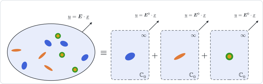
That picture is the mean-field approximation, and every scheme of this chapter is one answer to the question it leaves open: what is , and in which medium is each inclusion embedded? Taking   in the matrix gives the dilute estimate; requiring the matrix average to come out right gives Mori–Tanaka; embedding each phase in the unknown effective medium gives the self-consistent scheme.

2. What every scheme estimates

Under uniform boundary conditions the macroscopic strain and stress are the volume averages of their local counterparts,   and   (Hill, 1963). Linearity defines a strain concentration tensor per phase,   , and the two averages give

the sum over running over every phase and the one over over the phases other than the matrix, whose term vanishes in the second form. The effective tensor is thus known as soon as the concentration tensors are, and a scheme is precisely an estimate of them, built from the solution of an Eshelby problem posed in some reference medium.

The schemes below are written with three objects of Concentration, computed in the matrix unless stated otherwise. For an ellipsoidal phase of Hill tensor ,

The middle identity follows from         , and the last one from the definition       once         is noted. The second form of needs   to be invertible, the first one does not, and that is the one the package evaluates. The total dilute contributions are written

Cracks

A crack family is given by its density rather than by a volume fraction, which vanishes in the flat limit while the opening, and hence the strain the family carries, stays finite. The two products a scheme needs keep a finite limit:

with   for an elliptic family and for a ribbon family (Budiansky and O'Connell, 1976), and the compliance contribution derived in Crack opening displacement. The first limit is the strain carried by the openings per unit remote strain. The second follows because a traction-free crack carries no stress, so that    . A crack family therefore enters every scheme through these two terms, added to as    with      , and each page says where.

The concentration tensors of an estimate

Besides , a scheme estimates the concentration tensors of every phase, which concentration_tensors returns: the strain concentration tensor and the stress concentration tensor per unit macroscopic strain , such that

with    for a homogeneous phase. A crack family carries no stress,  , and its strain tensor is the limit of the previous section per unit density,     in the dilute case. Weighting each phase by , its volume fraction or the density of a crack family, every estimate of the package satisfies the two averages

and the stress-driven forms follow by composition with the effective compliance:    with   , and    . Relative to any reference stiffness , the contribution of phase to the estimate maps the macroscopic strain onto the mean polarization of the phase,

the last identity following from the two averages, and its compliance counterpart      maps the macroscopic stress onto   , with    . With the matrix as reference, reduces to the dilute for the dilute estimate, and to the dilute for the dual one; under any other scheme they carry the interactions that the scheme accounts for.

The one-site schemes all build these tensors in the same way. Phase solves its dilute problem in the reference medium of the scheme, loaded by a remote strain   that the scheme fixes,

and when the scheme singles out a matrix, the matrix takes the rest of the two averages. Each scheme page ends with its tensor , and Levin's theorem, at the end of the chapter, draws from the concentration tensors the response to free strains and prestresses.

3. The schemes at a glance

Each scheme answers the question of §1 differently. The table names the reference medium in which each inclusion is embedded, the field it is loaded by, and the page where the scheme is derived.

Scheme	Reference medium	Field applied to each inclusion	Page
Voigt	none	the macroscopic strain, in every phase	Bounds
Reuss	none	the macroscopic stress, in every phase	Bounds
Dilute	matrix	the macroscopic strain, at infinity	Dilute estimates
DiluteDual	matrix	the macroscopic stress, at infinity	Dilute estimates
MoriTanaka	matrix	the mean strain of the matrix	Mori–Tanaka
Maxwell	matrix	a remote strain applied to a domain holding every inclusion	Maxwell
PonteCastanedaWillis	matrix	the field inside the distribution ellipsoid of each pair of phases	Ponte Castañeda–Willis
SelfConsistent	effective medium, every phase	a remote strain fixed by the average	Self-consistent schemes
AsymmetricSelfConsistent	effective medium, inclusions only	a remote strain fixed by the average	Self-consistent schemes
DifferentialScheme	current effective medium	dilute increments	Differential scheme
Laminated	none, exact	piecewise-uniform fields	Laminate
ClusterModel	matrix	the remote strain and the field of every neighbor	Cluster model
EquivalentInclusion	matrix	a Galerkin polarization	Equivalent inclusion method

The pages of the chapter follow the order of the table. The bounds use no shape at all. The next four pages embed the inclusions in the matrix, each with a richer description of what surrounds them. The self-consistent and differential schemes then replace the matrix by the effective medium, the laminate is solved exactly, and the last two schemes resolve the interaction inclusion by inclusion. A last page, on Levin's theorem, applies to all of them.

4. Schemes that need positions

Every scheme of the table but the last two sees one inclusion in a reference medium and accounts for the others only through that reference: the interaction is treated in an average sense. The ClusterModel and the EquivalentInclusion method drop that one-site assumption and resolve the interaction inclusion by inclusion, which needs strictly more information than an RVE carries — the positions. They act on a ParticleAssembly instead, and share one ingredient, the two-inclusion interaction tensor . Both degenerate exactly onto Mori–Tanaka when the interaction is switched off, which is the sharpest available check that their assembly is right.

5. Number-type compatibility

The schemes involve nothing but tensor algebra and, for the iterative and differential ones, a solver, so that the scalar type is left open. Every scheme is mandated to support:

• Float64 — default;

• ForwardDiff.Dual — sensitivity analysis through fractions, moduli, geometric parameters;

• Complex{Float64} — frequency-domain viscoelasticity (parity with the C++ ECHOES library, templated on T = double | complex<double>);

• SymPyPythonCall.Sym, Symbolics.Num, BigFloat — best-effort, with explicit documentation of any limitation (the iterative SC solvers are not symbolic-friendly because the linear-system Jacobian must be numeric).

Where to go next

The schemes are now taken one at a time, starting with the two that need neither a shape nor a reference medium: Voigt and Reuss bounds. The tutorials A first homogenization and Bounds and classical schemes apply the schemes of this chapter to a first RVE, and the manual page Homogenization schemes gives their syntax.