
Highly conducting interfaces: equivalent conductivity vs. aspect ratio
The whole page as one script
Every block of this page, in order, is scripts/37_spheroid_hc_conductivity.jl. From a clone of the repository, julia --project=docs -e 'using Pkg; Pkg.instantiate()' once, then julia scripts/37_spheroid_hc_conductivity.jl, runs it end to end.
Before this page
The tutorial Imperfect interfaces: what they do to the local fields, where the highly conducting skin of an insulating particle is introduced at one aspect ratio, and the theory page Layered spheroid — confocal harmonic series, which gives the concentration tensors traced below.
The companion of The n-layer confocal spheroid: geometry and effective conductivity, which treats the low-conducting (Kapitza) interface. Here the interface is highly conducting — a surface layer of zero thickness and finite surface conductance
with
What the script computes. For an insulating particle carrying an HC interface, the equivalent particle conductivity
where
Because
Theory: Layered spheroid.
using MeanFieldHomogenization
using TensND
using Printf
using Plots
gr()

default(; left_margin = 5Plots.mm, bottom_margin = 5Plots.mm)
Setup
An insulating core (k₁ ≈ 0) isolates the interface contribution: whatever conductivity the particle ends up showing is carried entirely by its skin. The matrix is the unit-conductivity reference.
const KM = 1.0
const KCORE = 1.0e-8
const NSERIES = 6
const K0 = TensISO{3}(KM)
const KC = TensISO{3}(KCORE)
TensND.TensISO{2, 3, Float64, 1}
→ decomposition: (1.0e-8) 𝟏Build a one-layer spheroid of aspect ratio \omega at fixed transverse radius \rho_t = 1, carrying an HC interface of surface conductance k^{\mathrm s} (the code names them ϖ and β).
function _particle(ϖ, β; ρ_t = 1.0)
    ρ_a = ϖ * ρ_t
    return LayeredSpheroid(
        (ρ_a,), (ρ_t,), (KC,);
        interfaces = (MeanFieldHomogenization.SurfaceConductiveInterface(β),),
        Nseries = NSERIES,
    )
end
_particle (generic function with 1 method)k^eq from the volume-averaged concentration tensors. Both are transversely isotropic and diagonal in the spheroid frame, so the ratio is taken component-wise: index 1 is transverse, index 3 axial.
function _keq(ϖ, β)
    s = _particle(ϖ, β)
    A = gradient_gradient_concentration(s, KC, K0)
    B = flux_gradient_concentration(s, KC, K0)
    return real(B[1, 1] / A[1, 1]), real(B[3, 3] / A[3, 3])
end
_keq (generic function with 1 method)Aspect-ratio sweep
Oblate side
# The sphere `ϖ = 1` is excluded from both ranges: it has zero focal distance,
# so it is not a confocal spheroid at all and `LayeredSpheroid` rejects it
# ("use LayeredSphere"). The sweeps stop just short of it on either side.
const BETAS = (0.25, 0.5, 1.0, 2.0)
const OBL = exp10.(range(-1, -0.02; length = 40))
const PRO = exp10.(range(0.02, 1; length = 40))

function _curves(ϖs)
    kt = Dict{Float64, Vector{Float64}}()
    ka = Dict{Float64, Vector{Float64}}()
    for β in BETAS
        vt = Float64[]; va = Float64[]
        for ϖ in ϖs
            t, a = _keq(ϖ, β)
            push!(vt, t); push!(va, a)
        end
        kt[β] = vt; ka[β] = va
    end
    return kt, ka
end

kt_obl, ka_obl = _curves(OBL)
kt_pro, ka_pro = _curves(PRO)

println("HC (surface-conductive) interface on an insulating spheroid")
println("─"^70)
@printf "%-8s %12s %12s %12s %12s\n" "ϖ" "k_t (β=0.25)" "k_a (β=0.25)" "k_t (β=2)" "k_a (β=2)"
for (i, ϖ) in enumerate(OBL)
    (i - 1) % 13 == 0 || continue
    @printf "%-8.3f %12.4f %12.4f %12.4f %12.4f\n" ϖ kt_obl[0.25][i] ka_obl[0.25][i] kt_obl[2.0][i] ka_obl[2.0][i]
end
println()
println("Sanity checks:")
@printf "  β → 0 recovers the insulating particle : k_t = %.2e (expect ≈ %.0e)\n" _keq(0.5, 1.0e-9)[1] KCORE
println(
    "  k^eq grows monotonically with β at fixed shape :        ",
    all(kt_obl[0.25] .< kt_obl[2.0]) ? "OK" : "FAILED"
)
println()
HC (surface-conductive) interface on an insulating spheroid
──────────────────────────────────────────────────────────────────────
ϖ k_t (β=0.25) k_a (β=0.25) k_t (β=2) k_a (β=2)
0.100 3.6376 0.1396 28.6958 1.0291
0.212 1.7613 0.2545 13.9257 1.9337
0.450 0.8967 0.3908 7.1326 3.0782
0.955 0.5142 0.4953 4.1136 3.9622
Sanity checks:
β → 0 recovers the insulating particle : k_t = 1.33e-08 (expect ≈ 1e-08)
k^eq grows monotonically with β at fixed shape : OKGraphical output
Four panels: transverse and axial equivalent conductivity, over the oblate and the prolate range. The flat-particle limit is where the effect is strongest — a thin oblate platelet has a large surface-to-volume ratio, so its skin dominates.
function _panel(ϖs, curves, ttl, ylab; xlog = true)
    plt = plot(;
        xscale = xlog ? :log10 : :identity, yscale = :log10,
        xlabel = "aspect ratio ϖ = ρ_a / ρ_t", ylabel = ylab, title = ttl,
        legend = :best, size = (620, 460),
        left_margin = 10Plots.mm, bottom_margin = 5Plots.mm,
    )
    for (i, β) in enumerate(BETAS)
        plot!(plt, ϖs, curves[β]; label = "β = $β", lw = 2, color = i)
    end
    hline!(plt, [KM]; color = :grey, ls = :dash, label = "matrix k_m")
    return plt
end

p1 = _panel(OBL, kt_obl, "Oblate — transverse", "k_t^eq / k_m")
p2 = _panel(PRO, kt_pro, "Prolate — transverse", "k_t^eq / k_m")
p3 = _panel(OBL, ka_obl, "Oblate — axial", "k_a^eq / k_m")
p4 = _panel(PRO, ka_pro, "Prolate — axial", "k_a^eq / k_m")

p_full = plot(p1, p2, p3, p4; layout = (2, 2), left_margin = 8Plots.mm, bottom_margin = 8Plots.mm, size = (1250, 900))
p_full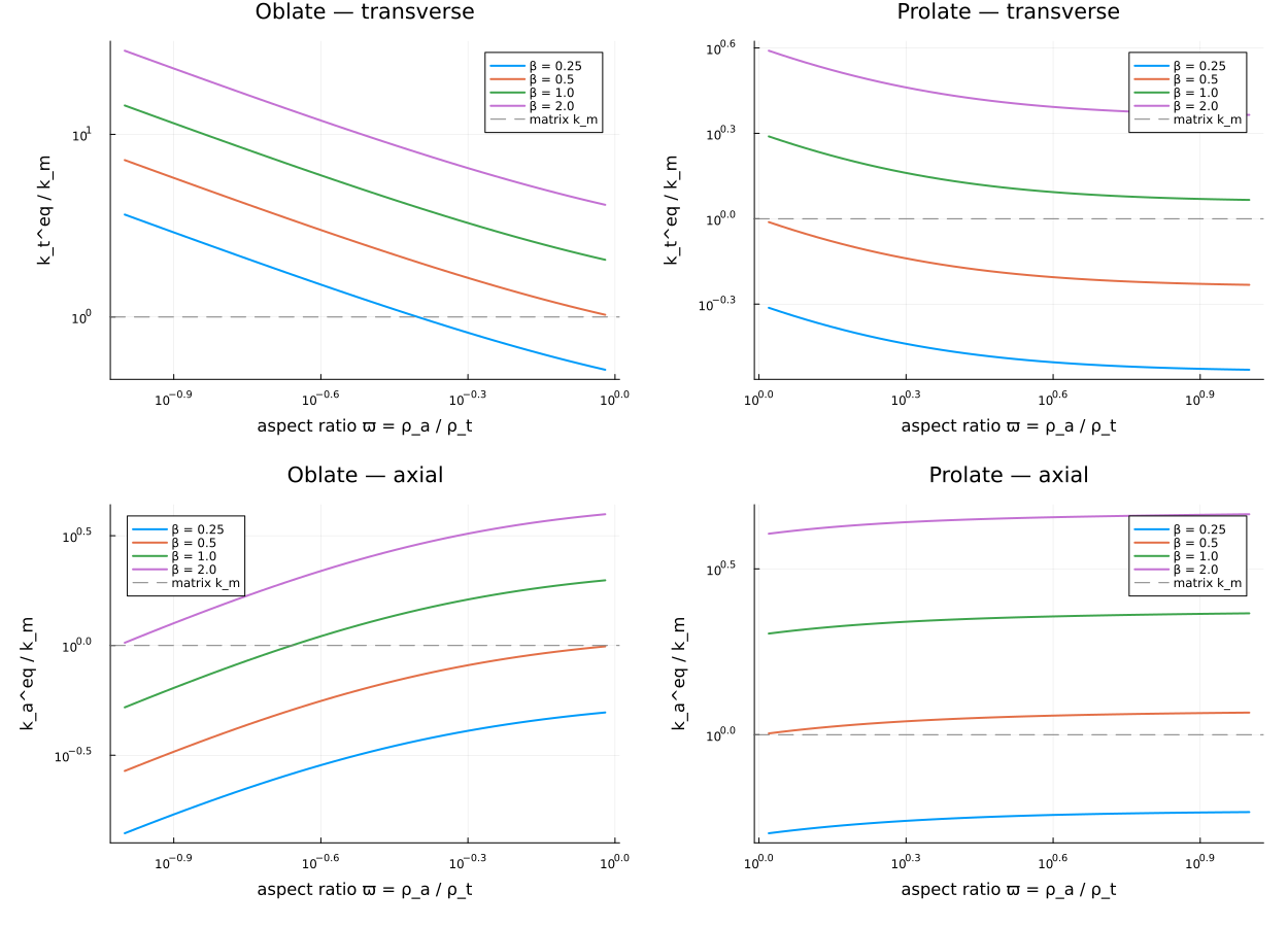
Effect on the effective conductivity of a composite
The equivalent particle is not just a diagnostic: it can be fed to any mean-field scheme as an ordinary homogeneous ellipsoid. Here a Mori–Tanaka estimate for aligned insulating platelets, with and without the HC skin.
const FRAC = 0.15
const OMEGA_PLATE = 0.1

function _khom(β)
    s = _particle(OMEGA_PLATE, β)
    rve = RVE()
    add_phase!(rve, :M, Ellipsoid(1.0, 1.0, 1.0), Dict(:K => K0); fraction = :rest)
    add_phase!(rve, :I, s, Dict(:K => KC); fraction = FRAC)
    K = homogenize(rve, MoriTanaka(), :K)
    return real(K[1, 1]), real(K[3, 3])
end

βsweep = range(0.0, 3.0; length = 30)
kh_t = Float64[]; kh_a = Float64[]
for β in βsweep
    t, a = _khom(β)
    push!(kh_t, t); push!(kh_a, a)
end

@printf "Mori–Tanaka, aligned platelets ϖ=%.2f at f=%.2f, insulating core:\n" OMEGA_PLATE FRAC
@printf "  β = 0 :  k_11/k_m = %.4f   k_33/k_m = %.4f\n" kh_t[1] / KM kh_a[1] / KM
@printf "  β = 3 :  k_11/k_m = %.4f   k_33/k_m = %.4f\n" kh_t[end] / KM kh_a[end] / KM
println(
    "  → the skin turns an obstacle into a conductor above β ≈ ",
    (idx = findfirst(kh_t .> KM); idx === nothing ? "never (in this range)" : @sprintf("%.2f", βsweep[idx]))
)

p_hom = plot(
    βsweep, kh_t ./ KM; label = "k₁₁ (in-plane)", lw = 2.5, color = :steelblue,
    xlabel = "surface conductance β", ylabel = "k^eff / k_m",
    title = "Mori–Tanaka: insulating platelets with an HC skin (f = $FRAC, ϖ = $OMEGA_PLATE)",
    legend = :topleft, size = (780, 480),
)
plot!(p_hom, βsweep, kh_a ./ KM; label = "k₃₃ (out-of-plane)", lw = 2.5, color = :darkorange)
hline!(p_hom, [1.0]; color = :grey, ls = :dash, label = "bare matrix")
p_hom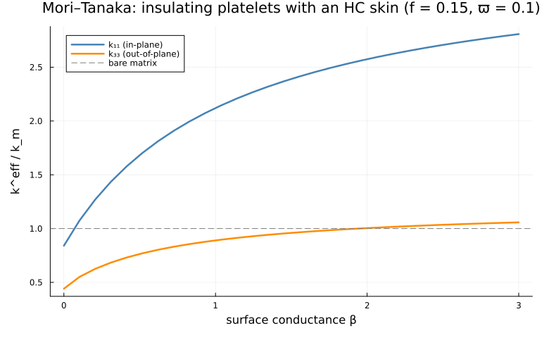
Where a curve crosses the dashed line, the insulating platelets and their skin conduct better, in that direction, than the matrix they replace.
Where to go next
The three spheroid pages rest on a closed form that requires confocal layers. A layered spheroid, meshed solves the same body by axisymmetric finite elements, calibrates the cell against the confocal solution, and then takes it to nests of freely chosen semi-axes that no closed form reaches.
This page was generated using Literate.jl.