The cluster model

Before this page

Two-inclusion interaction tensors, where the interaction tensor , its sign convention and the cluster truncation used below are set out, and Mori–Tanaka, onto which the model falls back when the interaction is switched off.

Every scheme of the previous pages sees one inclusion in a reference medium. The cluster model of Molinari and El Mouden (1996) is an N-body scheme instead: the mean strain of every inclusion is solved for, accounting for the pairwise interaction with each neighbor inside a cluster, on top of the interaction with the matrix. It acts on a ParticleAssembly, which carries the positions an RVE does not.

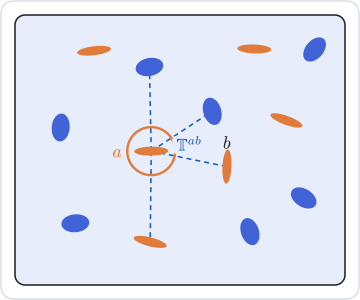
Notation as in the Nomenclature; the interaction tensor and the Green operator are defined on the interaction page.

1. From the integral equation to a linear system

Take the matrix, of stiffness and volume fraction , as reference, write    for the stiffness contrast of inclusion , and assume the strain uniform in each inclusion. Averaging the Lippmann-Schwinger equation over inclusion gives

and relating to the macroscopic strain through the average of the same equation yields

The paper's own sign is the opposite one

Molinari and El Mouden (1996) writes these two equations with a in front of the interaction sum, because their is the opposite of this package's (their self term is   ). The equations above are theirs with that single flip applied — see the convention note. Nothing else in this page or in the implementation carries a compensating sign.

Two identities connect this to the rest of the package:

the self term of the interaction family being the Hill tensor, and the far-field operator being the Hill tensor of the inclusion shape. For an isotropic matrix and spherical inclusions,

2. Families and the cluster

An infinite array is reduced to unknowns by taking a periodic elementary representative volume containing inclusions. Each inclusion of the cell carries a family of periodic images, all subjected to the same fields, and the sums are truncated to the images lying within a cluster radius of the receiver:

being the cluster attached to and the family . Convergence as   is proved in their Appendix B — see the cutoff discussion of Two-inclusion interaction tensors §7.

3. The block system

Splitting out of the sum and writing    turns the above into a linear system whose unknowns are order-4 tensors:

A single expression covers both the diagonal and the off-diagonal block, which is the practical dividend of the convention adopted here: in the opposite one the two cases carry opposite signs and have to be written separately.

The matrix concentration follows from the strain average rule and the effective stiffness from the stress one:

The implementation flattens the system onto the Kelvin-Mandel basis — where becomes an ordinary matrix product — and solves it with one dense factorization, rather than reproducing the tensorial Gauss elimination of the paper.

The unknowns of the system are therefore the concentration tensors themselves, and concentration_tensors returns them in the form of the overview: one strain tensor per family, keyed :family_<label>, with   , and the matrix closing both averages as above.

4. The Mori-Tanaka limit

Reduce the cluster to its own receiver. Every vanishes and

which is the Mori-Tanaka system term by term.

An exact degeneracy, not an approximation

With cluster_radius = 0 the cluster model is MoriTanaka, as an algebraic identity — Appendix C of Molinari and El Mouden (1996). The test suite checks it to machine precision, for one family and for two, in elasticity and in conduction. It is the sharpest available statement that the assembly of is right.

5. What the cluster buys

Since has no isotropic part (Two-inclusion interaction tensors §4), the correction is purely deviatoric:

• the effective bulk modulus of a cubic array equals the Mori-Tanaka one exactly;

• the effective shear moduli do not, and the array is cubic, not isotropic — the two shear constants differ;

• for a statistically isotropic arrangement the orientation average of vanishes and the model collapses back onto Mori-Tanaka. The cluster model is therefore a statement about anisotropic or specific arrangements, which is why it needs a ParticleAssembly rather than an RVE.

Their own results, reproduced in scripts/91: the estimate is flat beyond   periods; Mori-Tanaka overestimates the shear modulus of a simple-cubic array of stiff spheres, so it is not a bound for that distribution; and at equal volume fraction the SC, BCC and FCC arrangements differ, the simple-cubic one being the softest.

Where to go next

The next page, The equivalent inclusion method, poses the same problem as a Galerkin discretization, which reduces to the system of §3 under periodic boundary conditions and adds a rigorous bound to the estimate. The results of Molinari and El Mouden (1996) quoted in §5 are reproduced in The cluster model on cubic arrays, and the construction of a ParticleAssembly is described in Particle assemblies and N-body schemes. The API entries are in API — Particle assemblies.