Bounds and classical schemes

Before this page

The tutorial A first homogenization, whose RVE and dilute and Mori–Tanaka estimates are reused below, and the theory page Homogenization schemes, whose pages derive the bounds and the iterative schemes.

The dilute and Mori–Tanaka estimates of the previous tutorial are two points in a much larger family. This page places every classical scheme on a single graph, bracketed by the two estimates that must bound any physically admissible effective stiffness: the Voigt and Reuss bounds.

Rigorous bounds

For a composite with phases at volume fractions , the Voigt bound assumes a uniform strain throughout the RVE, and the Reuss bound a uniform stress:

Both are exact bounds — no assumption on the microstructure's geometry is needed — and order every physically realizable effective bulk modulus (Hill, 1952; Hill, 1963):

Estimates between the bounds

Self-consistent

SelfConsistent drops the "matrix" altogether: every phase is embedded directly in the effective medium itself, and the effective stiffness must satisfy the implicit condition

Budiansky and O'Connell (1976), solved by a damped Picard iteration internally (abstol, maxiters control its convergence). This is the natural model for an interpenetrating, polycrystal-like microstructure where no phase plays the role of a continuous matrix.

Differential

DifferentialScheme builds the composite incrementally, re-homogenizing after each infinitesimal addition of inclusions — see the dedicated tutorial for the full picture.

Putting them on one graph

using MeanFieldHomogenization
using TensND
using LinearAlgebra
using Plots
gr()  # headless backend; GKSwstype is set to "100" in make.jl

C_m = iso_stiffness(30.0, 10.0)   # matrix
C_i = iso_stiffness(60.0, 20.0)   # stiffer inclusion

function build(f)
    r = RVE()
    add_phase!(r, :M, Ellipsoid(1.0), Dict(:C => C_m); fraction = :rest)
    f > 0 && add_phase!(r, :I, Ellipsoid(1.0), Dict(:C => C_i); fraction = f)
    return r
end

fs = collect(range(0.0, 0.6; length = 25))
schemes = [
    (Voigt(), "Voigt", :red, :dash),
    (Reuss(), "Reuss", :red, :dot),
    (Dilute(), "Dilute", :blue, :solid),
    (MoriTanaka(), "MoriTanaka", :green, :solid),
    (SelfConsistent(; abstol = 1.0e-10, maxiters = 200), "SelfConsistent", :purple, :solid),
    (DifferentialScheme(; nsteps = 100), "Differential", :orange, :solid),
]

plt = plot(;
    xlabel = "inclusion volume fraction f", ylabel = "k_eff",
    legend = :topleft, framestyle = :box, size = (760, 480),
)
for (sch, label, color, ls) in schemes
    ks = [k_mu(homogenize(build(f), sch, :C))[1] for f in fs]
    plot!(plt, fs, ks; label = label, color = color, linestyle = ls, lw = 2)
end
plt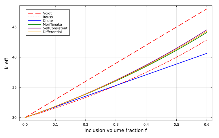

At f = 0.3, the numbers behind the plot:

rve = build(0.3)
for (sch, label, _, _) in schemes
    k, _ = k_mu(homogenize(rve, sch, :C))
    println(rpad(label, 16), round(k, digits = 4))
end

Voigt           39.0
Reuss           35.2941
Dilute          35.3182
MoriTanaka      36.0622
SelfConsistent  36.1975
Differential    36.1276

Every estimate lies between the Voigt and Reuss bounds — Voigt above, Reuss below, everything else in between. This is the central point of mean-field homogenization: the choice of scheme is not a numerical detail but a modeling decision about the microstructure's topology (matrix-inclusion vs. interpenetrating, dilute vs. dense, aligned vs. random).

Where to go next

Every scheme above rests on the Hill tensor of its inclusions, computed out of sight. Hill polarization tensors in practice opens the tutorials on the problem of a single heterogeneity by computing that tensor explicitly. The schemes come back after those, starting from the limit opposite to the stiff inclusions above, a phase whose stiffness vanishes: Porous materials: the self-consistent trap and every scheme. The differential scheme, only sketched here, has its own tutorial, The differential scheme and path dependence.