MeanFieldHomogenization.jlEffective properties of heterogeneous materials

What it does ​

Given a reference medium and an inclusion shape, MeanFieldHomogenization builds the Hill polarization tensor (Eshelby's result), derives the concentration tensor for each phase, and assembles a homogenization scheme — dilute, Mori–Tanaka, self-consistent, differential, PCW, or the classical bounds — into an effective stiffness or conductivity.

That chain is the whole library. The reading path follows it: first the problem of a single heterogeneity, an ellipsoid, a crack or a layered pattern; then the schemes that assemble those solutions, one family per page, from the bounds to the N-body schemes that resolve the interaction inclusion by inclusion; and finally the chain generalized in one direction at a time, a different physics for transport and a different time dependence for viscoelasticity.

MeanFieldHomogenization is a pure-Julia reimplementation of the Eshelby/Hill machinery of the Echoes C++/Python codebase; see From Echoes to MeanFieldHomogenization for the translation guide.

Installation ​

pkg> add MeanFieldHomogenization

Nothing else has to be installed by hand for numerical work, derivatives included.

A first calculation ​

A porous solid, and every scheme the package ships, against the bounds that frame them. The void is given a small but non-zero stiffness, which is what lets the self-consistent branch stay on the physical solution:

using MeanFieldHomogenization, TensND, Plots
gr()  # headless backend; GKSwstype is set to "100" in make.jl

C_solid = iso_stiffness(90.0, 30.0)     # GPa
C_void  = iso_stiffness(0.01, 0.005)

function bulk(f, scheme)
    r = RVE()
    add_phase!(r, :M, Ellipsoid(1.0), Dict(:C => C_solid); fraction = :rest)
    f > 0 && add_phase!(r, :V, Ellipsoid(1.0), Dict(:C => C_void); fraction = f)
    return first(k_mu(homogenize(r, scheme, :C)))
end

fs = range(0.0, 0.5; length = 61)
schemes = ("Voigt" => Voigt(),
           "Reuss" => Reuss(),
           "Mori-Tanaka" => MoriTanaka(),
           "Dilute (dual)" => DiluteDual(),
           "Self-consistent" => AsymmetricSelfConsistent(; abstol = 1.0e-10,
                                                           maxiters = 200,
                                                           select_best = true),
           "Differential" => DifferentialScheme(; nsteps = 100))

plt = plot(; xlabel = "porosity f", ylabel = "effective bulk modulus k [GPa]",
             legend = :topright, framestyle = :box, size = (760, 470))
for (name, s) in schemes
    plot!(plt, fs, [bulk(f, s) for f in fs]; label = name, lw = 2)
end
plt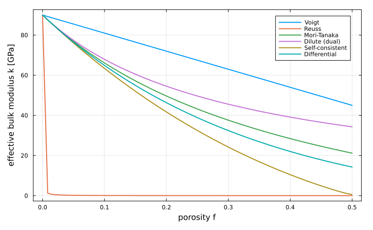

Voigt and Reuss bracket the others; the three estimates between them differ by how much of the load each void is assumed to see. Porous materials works through why the standard self-consistent scheme fails on this problem and what replaces it, and Getting started takes a single estimate more slowly, defining each object on the way.

Reading paths ​

The documentation is organized by the question each chapter answers. Theory explains why an estimate is the right one, the Manual describes how each kind of object is written, the Tutorials drive a calculation from start to finish, and the Applications build complete models of real materials. Three entry points follow from it, depending on what the reader already knows.

New to mean-field homogenization. The chapter Theory is written for this reader and is best read in the order it states, from The Eshelby inclusion problem to Homogenization schemes, which together contain the whole chain that the rest generalizes. The tutorial A first homogenization then puts it to work.

Knowing what is to be computed. Getting started and Schemes and RVEs are enough to write a first model; the Manual then has one page per morphology, from Ellipsoidal inclusions to Neural-surrogate inclusions, and the Applications, from Multiscale elasticity of a hydrating cement paste onwards, show complete models.

Coming from Echoes. The correspondence between the two libraries, class by class, is in From Echoes to MeanFieldHomogenization, and echoes2mfh translates an existing script.

The symbols. Every symbol of the formulas is listed in the Nomenclature, with its meaning and its unit. Hovering an equation on any page shows the symbols it holds, with their meaning on that page.