Damage by the growth of microcracks

The whole page as one script

Every block of this page, in order, is scripts/material_laws/15_crack_damage.jl. From a clone of the repository, julia --project=docs -e 'using Pkg; Pkg.instantiate()' once, then julia scripts/material_laws/15_crack_damage.jl, runs it end to end.

In most damage models, a scalar variable degrades the stiffness through a function chosen to fit tests. This page derives a damage law from the microstructure instead. The variables are the densities of the families of microcracks that the solid contains, the stiffness is the homogenized stiffness of the cracked solid, and the evolution follows from an energy balance on the cracks. The approach is that of Dormieux and Kondo (2016), applied by Dormieux et al. (2006) to fluid-saturated media. The example below runs the law.

State and energy

A linear elastic solid of stiffness contains families of penny-shaped cracks, family having the density and a given orientation (or an isotropic distribution of orientations). The cracks are open and their faces carry no traction. At fixed densities the cracked solid is linear elastic, with the stiffness that a scheme of the package gives, . Its free energy per unit volume is

The stress and the force conjugate to each density follow from it:

is the energy released per unit increase of the density at fixed strain: the force that drives the growth of the family. The dissipation is  , and it is nonnegative because cracks only grow ( ) and because a crack can only soften the solid ( ).

What drives a family

When the compliance of the cracked solid is affine in the densities,    , as with the Mori–Tanaka scheme, the derivative of the stiffness is     . The driving force then takes a form that shows what drives it:

acts on the traction   that the stress applies to the plane of the family. A family is driven by the normal and the shear tractions on its own plane, and a family whose plane carries no traction does not grow, however large the stress. This is what makes the damage anisotropic, as the families loaded differently grow differently. The law itself does not rely on this form: it differentiates by automatic differentiation through the scheme, whatever the scheme.

The criterion and the resistance

A family grows when its driving force reaches a resistance :

These are the conditions of a rate-independent process. Either the family keeps its density, below the criterion, or it grows while staying on it.

The resistance follows from the fracture of the cracks themselves when the family is cracks per unit volume that grow in size at fixed number. With their radius, the density is  . Griffith's criterion (Griffith, 1921) states that a crack front advances when the energy released per unit area of new crack surface reaches the toughness . When the radius of every crack grows by , the crack surface created per unit volume is   , and it costs the energy    . The density grows by   , which releases  . Equating the two:

and being the radius and the density in a reference state, which fix  . This is CrackGrowthResistance. Any other function of the density can be given instead, for instance a resistance that increases with the density to represent obstacles that the cracks meet as they grow.

Stability

Under a fixed strain, a family on its criterion keeps growing if a small increase of its density raises the driving force more than the resistance, that is, if    at fixed strain. The growth is then unstable. With Griffith's resistance is negative: once the criterion is reached, the density jumps to a larger value, the first one where the driving force has fallen back to the resistance, and the stress drops. A resistance that increases fast enough makes the growth stable and the damage progressive.

An unstable growth is also a numerical difficulty. Newton's method, started from the densities of the last step, cannot jump to a distant root. A small viscosity regularizes it:

Above the criterion the density now grows at a finite rate, so a step short against changes it little. As becomes small against the duration of the loading, the response tends to the rate-independent one, jump included. The regularization is the keyword τ of CrackGrowthDamage.

The law in MaterialLaws

CrackGrowthDamage builds a ResidualLaw whose internal variables are the densities. Over a step from it solves, for every family, one of the two following equations:

The first is the complementarity of the growth and of the criterion: its root either keeps the density or puts the family on its criterion. Both terms are dimensionless, so that they compare. A step is elastic, and the densities are kept, when every family is below its criterion at the densities of the last step.

The consistent tangent comes, as for any law of the chapter, from the implicit-function theorem applied to these equations. It contains the softening due to the growth of the cracks during the step. A density must stay positive; a Newton correction that leads to a negative density is halved until it does not.

Scope

cracks	penny-shaped, open, with traction-free faces: no unilateral contact, no friction
families	any number, oriented or isotropically distributed; each its own resistance
schemes	any linear scheme of the package that handles cracks
softening	a softening law localizes in a structure; the response of a finite-element computation then depends on the mesh, which a point computation does not show

Example: damage by the growth of microcracks

This example runs the damage law derived from the microcracks of a brittle solid. It compares a progressive damage with the unstable growth that Griffith's criterion gives, and it shows how a viscosity regularizes the latter.

The cracked solid

A rock-like solid (bulk modulus 30 GPa, shear modulus 20 GPa) contains penny-shaped microcracks of all orientations, of initial density  . The stiffness of the cracked solid is the Mori–Tanaka one, as for a linear computation:

using MeanFieldHomogenization, TensND, Plots

k, μ = 30e3, 20e3                                                 # MPa
C₀ = TensISO{3}(3k, 2μ)
rve = RVE()
add_phase!(rve, :M, Ellipsoid(1.0), Dict(:C => C₀); fraction = :rest)
add_phase!(rve, :F, PennyCrack(1.0), Dict(:C => C₀); density = 0.05, symmetrize = :iso)

symmetrize = :iso spreads the family over every orientation, so that the solid stays isotropic as the cracks grow.

Progressive damage

A first resistance increases with the density, as if the cracks met obstacles while they grow:

rising(d) = 0.04 * (1 + 20 * (d - 0.05))                          # MPa
progressive = CrackGrowthDamage(rve; resistance = rising)

code	theory
rve	the cracked solid; the density of the crack phase is the initial one
resistance	the resistance that the driving force must reach
CrackGrowthDamage	the law whose internal variable is the density of each family

The bar is pulled, unloaded to zero strain, then pulled further. Its lateral faces are free.

ε_axial(t) = t < 0.5 ? 3e-3 * t / 0.5 : t < 0.7 ? 3e-3 * (0.7 - t) / 0.2 : 4e-3 * (t - 0.7) / 0.3
r = point_response(progressive, LoadingPath(range(0, 1; length = 61); ε11 = ε_axial))

p1 = plot(r[:ε11] * 1e3, r[:σ11]; lw = 2, label = "", xlabel = "axial strain (‰)", ylabel = "axial stress (MPa)")
p2 = plot(r[:ε11] * 1e3, r[:F]; lw = 2, label = "", xlabel = "axial strain (‰)", ylabel = "crack density d")
plot(p1, p2; layout = (1, 2), size = (760, 320), left_margin = 3Plots.mm, bottom_margin = 4Plots.mm)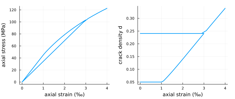

The response is linear until the driving force reaches the resistance, near 1 ‰. The cracks then grow, and the stress bends under its linear trend. On unloading the density is kept: the stress returns to the origin along a straight line, whose slope is the stiffness of the more cracked solid. On reloading, the density grows again only past the largest strain reached before. Nothing in this response was fitted except the resistance. The loss of stiffness is what the homogenization gives for the density reached.

Unstable growth, regularized

Griffith's resistance, for cracks of initial radius 1 mm and a toughness of 20 J/m², decreases as the cracks grow:

griffith = CrackGrowthResistance(; Gc = 0.02, a₀ = 1.0, d₀ = 0.05)   # N/mm, mm

The growth is then unstable: at the threshold the density jumps. A rate-independent law cannot follow the jump from the density of the last step, so the growth is regularized by a time , compared here with the duration of the loading (one unit of time):

path = LoadingPath(range(0, 1; length = 41); ε11 = t -> 2e-3 * t)
p1 = plot(; xlabel = "axial strain (‰)", ylabel = "axial stress (MPa)", legend = :bottomright)
p2 = plot(; xlabel = "axial strain (‰)", ylabel = "crack density d", legend = :topleft)
for τ in (1.0, 0.1, 0.01)
    rτ = point_response(CrackGrowthDamage(rve; resistance = griffith, τ), path)
    plot!(p1, rτ[:ε11] * 1e3, rτ[:σ11]; lw = 2, label = "τ = $τ")
    plot!(p2, rτ[:ε11] * 1e3, rτ[:F]; lw = 2, label = "τ = $τ")
end
plot(p1, p2; layout = (1, 2), size = (760, 320), left_margin = 3Plots.mm, bottom_margin = 4Plots.mm)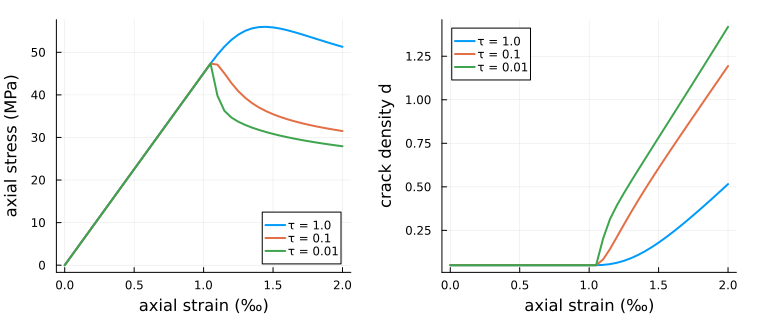

With the largest the cracks grow slowly and the stress keeps rising for a while past the threshold. As decreases, the curves approach the rate-independent response: the density jumps at the threshold, and the stress drops at once to the value that the more cracked solid carries. The peak stress is the same for   and  , the threshold of the rate-independent law; the response after the peak still moves with , and a smaller needs shorter steps, which the driver takes by cutting those that fail.

Checks

The tangent is consistent. The contract checker compares the tangent from the implicit-function theorem with the derivative of the stress, on a damaging step:

check_material_interface(progressive; verbose = false)

true

Below the threshold, the law is the linear cracked solid. Its tangent is then the Mori–Tanaka stiffness at the initial density:

σ, 𝕂, _ = point_update(progressive, Mandel{Float64}(2e-4, -1e-4, 0, 1e-4, 0, 0), initial_state(progressive), 1.0)
𝕂 ≈ KM(homogenize(rve, MoriTanaka(), :C))

true

Going further

• Oriented families (cracks with a given normal, without symmetrize) grow each under the tractions on their own plane, so that the damage becomes anisotropic. Each family may have its own resistance: resistance = (F1 = R₁, F2 = R₂).

• The law is a law of MaterialLaws and runs at the quadrature points of a finite-element computation. A softening law localizes in a structure, and the finite-element response then depends on the mesh.

---

This page was generated using Literate.jl.