FEniCSx backend

Before this page

Materials, for what a material computes at a quadrature point, and Ferrite backend, for the pieces of the coupling that belong to the package whatever the finite-element code.

FEniCSx writes a problem in UFL and assembles it in C++; the Python package mfh_fenicsx, in python/mfh_fenicsx of the repository, lets the stress of such a problem be a material of this package: a law of MaterialLaws, a nonlinear composite, a polycrystal. Julia runs inside the Python process, through juliacall.

In short

1. Install Julia with this package, and Python with dolfinx and mfh_fenicsx.

2. Write the residual of your problem in UFL with stress.sigma where the stress goes (A load step).

3. Let Newton and quasistatic run the steps; read the stresses, the reactions and the internal variables.

Every law of MaterialLaws works this way, a homogenized composite or a polycrystal as well as J2 plasticity, and so does a poroelastic material in a coupled displacement–pressure problem (A coupled problem).

How it works

The stress is an external operator of dolfinx-external-operator (Latyshev et al., 2025): a UFL object that stands for in the forms, and whose values and derivative are supplied, at every quadrature point, by a Python function. The residual is written with it as with any stress,

and its Jacobian is the derivative of the operator, the consistent tangent  .

At each Newton iteration the strains of all the quadrature points are evaluated in one array and handed to Julia in one call, update_points!, which computes every stress and every tangent from the states of the last converged step, on as many threads as Julia has, and writes them into arrays that NumPy reads without a copy. The tangent the Jacobian asks for is the one of that call: no point is integrated twice. The states stay in Julia, in a QuadratureStates, and a step is committed or rolled back as with Ferrite.

Python (mfh_fenicsx)	Julia
mf.start()	starts Julia, loads the package; installs nothing
Material(material, ncells, nqp)	the material and its QuadratureStates
Stress(material, u)	the external operator and its quadrature space
Poroelastic(material, u, p)	the operators and of a coupled problem
Newton(stress, residual, u, bcs)	Newton's method on one step; MUMPS when PETSc has it
quasistatic(newton, times, prescribe)	the steps, a failing one halved, as quasistatic!
stress.commit(), stress.rollback()	commit!, rollback!
newton.reaction(dofs)	the force of a Dirichlet condition
stress.material.internal("p")	the committed values of an internal variable

Installation

Two environments meet: a Julia project that holds this package and PythonCall, and a Python environment that holds dolfinx and mfh_fenicsx. Nothing is downloaded at run time: both are prepared once.

1. Julia and its project. Install Julia with juliaup, then create a project with the two packages:

julia --project=$HOME/mfh-fenicsx-julia -e 'using Pkg; Pkg.add(["MeanFieldHomogenization", "PythonCall"])'

2. Python with dolfinx. dolfinx comes from conda-forge; the other packages from PyPI, and mfh_fenicsx from the repository of this package:

conda create -n fenicsx -c conda-forge python=3.12 fenics-dolfinx=0.10 mpich python-gmsh matplotlib-base pip
conda activate fenicsx
pip install dolfinx-external-operator==0.10.2 juliacall==0.9.37
pip install -e path/to/MeanFieldHomogenization.jl/python/mfh_fenicsx

3. The environment of each session. Tell juliacall which Julia and which project to use, how many threads Julia has, and leave the other libraries one thread each:

export PYTHON_JULIAPKG_EXE=$(which julia)               # the Julia to embed
export PYTHON_JULIAPKG_PROJECT=$HOME/mfh-fenicsx-julia  # the project of step 1
export PYTHON_JULIACALL_THREADS=4                        # Julia's threads
export OPENBLAS_NUM_THREADS=1 OMP_NUM_THREADS=1          # no threads competing with Julia's

The direct solver, MUMPS, factorizes with OpenMP threads when it may; their sums change order from one run to the next, so that two runs differ in the last digits. One OpenMP thread keeps the runs reproducible and leaves the cores to Julia.

4. A check. This starts Julia, loads the package (a few seconds the first time, while Julia compiles) and prints Julia's threads:

python -c "import mfh_fenicsx as mf; jl = mf.start(); print(jl.Threads.nthreads())"

A load step

The code below is the core of every example: a displacement field, the material at its quadrature points, the residual, and the steps.

import numpy as np
import ufl
from dolfinx import fem, mesh
from mpi4py import MPI

import mfh_fenicsx as mf
from mfh_fenicsx.fem import Newton, Stress, quasistatic, strain

mf.start()
domain = mesh.create_unit_cube(MPI.COMM_WORLD, 4, 4, 4)
V = fem.functionspace(domain, ("Lagrange", 1, (3,)))
u = fem.Function(V)

# The material, written in Julia; any material of the package goes there.
stress = Stress("J2Plasticity(; E = 200.0e3, ν = 0.3, σ₀ = 250.0, H = 2.0e3)", u)
residual = ufl.inner(stress.sigma, strain(ufl.TestFunction(V))) * stress.dx

# Clamped at the bottom, the top pulled along z.
bottom = fem.locate_dofs_geometrical(V, lambda x: np.isclose(x[2], 0.0))
top_facets = mesh.locate_entities_boundary(domain, 2, lambda x: np.isclose(x[2], 1.0))
top = fem.locate_dofs_topological(V.sub(2), 2, top_facets)
pull = fem.Constant(domain, 0.0)
bcs = [fem.dirichletbc(np.zeros(3), bottom, V), fem.dirichletbc(pull, top, V.sub(2))]

# The top is pulled to 4e-3 over ten steps of a "time" t from 0 to 1.
def prescribe(t):
    pull.value = 4.0e-3 * t

newton = Newton(stress, residual, u, bcs)
quasistatic(newton, np.linspace(0.0, 1.0, 11), prescribe)
print(newton.reaction(top))   # the force on the top

The units are those of the numbers you give: here MPa for the moduli and a unit cube, so that the reaction is in MPa times the unit of area.

code	what it does
Stress(material, u)	builds the quadrature space, the states, and the operator stress.sigma
stress.dx	the measure whose quadrature matches the space of the stress; use it in the forms
Newton(...)	compiles the forms once; solve() runs one step
quasistatic(...)	a step that fails (Newton, or a point that does not integrate) is rolled back and halved
prescribe(t)	sets the boundary values at the time t; quasistatic calls it at each step
newton.reaction(top)	the force that the condition on top exerts, summed over its degrees of freedom

A coupled displacement–pressure problem

A poroelastic material (BiotPoroelasticity, ClosingCrackPoroelasticity) depends on the strain and on the pore pressure , and gives the stress and the fluid content . The problem then has two unknowns, and , in a mixed space, and two balances: of the solid, with , and of the fluid, with the change of over the step and Darcy's flow,

import basix.ufl
from mfh_fenicsx.fem import Poroelastic

cell = domain.basix_cell()
W = fem.functionspace(domain, basix.ufl.mixed_element([
    basix.ufl.element("Lagrange", cell, 2, shape=(3,)),   # u, quadratic
    basix.ufl.element("Lagrange", cell, 1),               # p, linear
]))
w = fem.Function(W)
u, p = ufl.split(w)
v, q = ufl.TestFunctions(W)

poro = Poroelastic("BiotPoroelasticity(; E = 10.0e3, ν = 0.25, b = 0.8, M = 5.0e3)", u, p)
dt = fem.Constant(domain, 1.0)
mobility = 1.0e-3                                          # k/μ
residual = (
    ufl.inner(poro.sigma, strain(v)) * poro.dx             # + the loads
    + (poro.phi - poro.phi_old) * q * poro.dx
    + dt * mobility * ufl.dot(ufl.grad(p), ufl.grad(q)) * poro.dx
)

poro.phi_old is the fluid content at the end of the last committed step: it is updated by poro.commit(). The time step must be the same in the material and in the residual: set dt.value in prescribe, from poro.dt, which quasistatic sets before calling it. The test of Terzaghi's consolidation and the borehole example below are complete programs of this kind.

Conventions

• Components. The stress and the strain cross the boundary in Kelvin–Mandel components, ordered    , the package's convention; mandel_from_tensor, tensor_from_mandel and tensor4_from_mandel convert from and to full tensors.

• Points. The points are ordered cell by cell, as a quadrature space of dolfinx orders them; the ghost cells of a process are included.

• Two dimensions mean plane strain: the material is integrated in three dimensions with    , and the out-of-plane stress is kept in stress.material.stress[2]. Axisymmetry is not covered yet.

• Poroelastic materials, of gradients and fluxes (BiotPoroelasticity, ClosingCrackPoroelasticity), go to Poroelastic(material, u, p): its sigma and phi are two external operators on the same operands, whose values and derivatives come from one Julia call; phi_old holds the fluid content of the last committed step, for the storage term of the balance of the fluid.

• Processes. The tests and the examples run on one MPI process; Julia's threads do the parallel work of the materials.

gmsh and Julia's signals

Julia stops its threads at safepoints through the signal SIGSEGV. gmsh.initialize() resets SIGSEGV, SIGBUS, SIGILL, SIGFPE (and SIGINT) to their defaults, and the next garbage collection on several threads then kills the process without a message. mfh_fenicsx saves Julia's handlers when it starts and puts them back before every call into Julia and at exit. After such a library, call mfh_fenicsx.restore_signals() before calling Julia yourself.

Common problems

what happens	why, and what to do
juliacall downloads Julia or packages, or cannot find the package	PYTHON_JULIAPKG_EXE or PYTHON_JULIAPKG_PROJECT is not set: see step 3 of the installation
the first step takes seconds, the next ones milliseconds	Julia compiles the material on its first call; it is paid once per session
JuliaError: LocalIntegrationError	a point could not follow the step; quasistatic halves the step by itself, Newton.solve alone does not
NewtonError	the step is too large for the material, or the tangent is not consistent; use smaller steps or quasistatic
the process dies without a message after gmsh.initialize()	see the warning on signals above
two runs differ in the last digits	set OMP_NUM_THREADS=1 (step 3)
Stress refuses the material	it is not purely mechanical: a poroelastic material goes to Poroelastic

What is checked

The tests of python/mfh_fenicsx/tests compare the coupling with references that do not go through it:

test	reference	agreement
a homogeneous strain on a cube, 3-D and plane strain	Hooke's law; Julia's single-point update along a plastic path	to round-off
a plastic cube, clamped and pulled, the same hexahedral mesh and quadrature	the package's Ferrite adapter	nodal displacements to of the pull
a cube of a Mori–Tanaka composite of tilted spheroids	a dolfinx solve written in UFL with the homogenized stiffness
the thick cylinder under pressure, plane strain	Lamé's closed form	second-order convergence
a heterogeneous plastic problem	the order of convergence of Newton's method	about 2; an elastic tangent does not converge
Terzaghi's consolidation of a column, linear Biot law, mixed	the Fourier series of the one-dimensional diffusion	a few percent of the undrained pressure, halved with the time step (backward Euler)

Examples

Each example is a script of python/mfh_fenicsx/examples, which writes its results and its figure in the directory --out; examples/run_all.sh runs them all and copies the figures and the results (*.json) here. The times below were measured on 8 logical CPUs (AMD EPYC-Milan), Julia on 4 threads unless stated.

A plate with a hole in a fiber composite

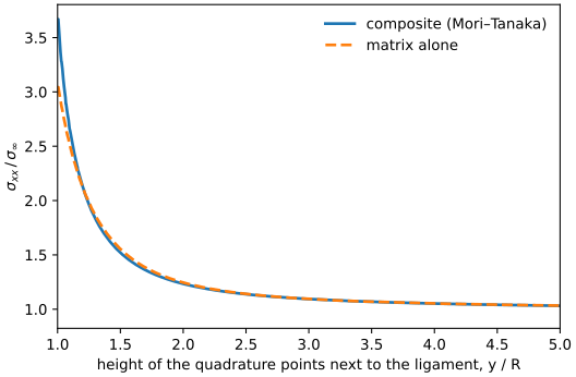
01_plate_with_hole.py. A plate with a hole, in plane strain, of an epoxy reinforced by 30 % of glass spheroids aligned with the load, whose Mori–Tanaka stiffness the package computes. The material at every point gives the displacements of a dolfinx solve with the homogenized stiffness written in UFL, to better than ; the stress concentration at the hole rises from 3.04 for the matrix alone to 3.65.

A notched plate whose microcracks grow

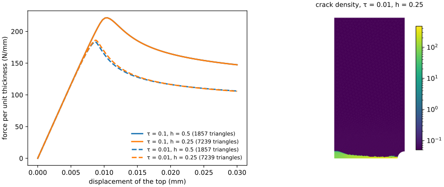
02_notched_plate_crack_growth.py. Penny-shaped microcracks of all orientations grow at Griffith's resistance, which decreases as they grow; the growth is regularized by a viscosity of time (CrackGrowthDamage). With   (the loading lasts 1) two meshes give the same curve; with   the cracks grow in a band along the ligament and the meshes start to part, by about 1 % on the peak. The law is local: as decreases the band follows the elements, which no mesh refinement cures.

A borehole in a rock whose cracks close

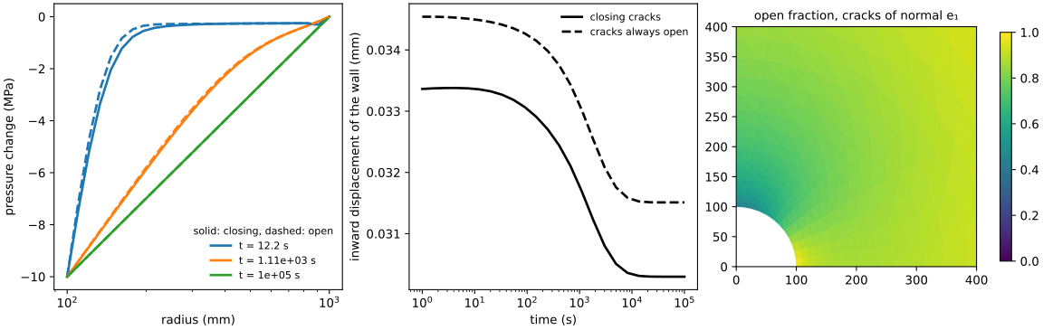
03_borehole_closing_cracks.py. A saturated rock holds three families of microcracks, of normals , , , which close as the effective stress compresses them across their planes (ClosingCrackPoroelasticity). The pressure in a borehole is lowered by 10 MPa and held; the problem is the coupled one, in plane strain. Around the hole the effective stress rises and the cracks whose normal is tangential to the wall close (down to 42 % open), which stiffens the rock: the wall moves less than with cracks that stay open. At the end the flow is steady, and the pressure is that of a radial flow,  , to   MPa. The mobility of the fluid is constant here: this law does not let the permeability follow the apertures.

A polycrystalline plate: Kröner and Hill

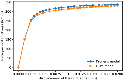
04_polycrystal_plate.py. Every point is an aggregate of eight viscoplastic crystals of random orientations (Polycrystal), whose grains share the strain as KronerModel or HillModel says. Hill's aggregate, constrained by its own flowing tangent, carries less load than Kröner's, constrained by the elastic aggregate. These materials are costly: on 151 triangles, 109 s with Kröner's model and 440 s with Hill's.

Creep of a composite beam

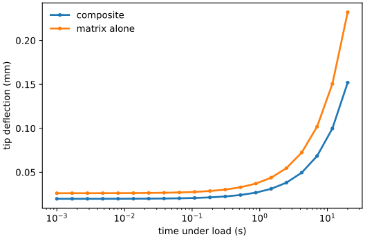
05_composite_beam_creep.py. A cantilever of a matrix that creeps by Norton's law, reinforced by 20 % of particles, under a load held for 20 s; the composite is homogenized at every point by QuasiElasticComposite (Brenner et al., 2002). The first deflection of the matrix alone is the elastic one of beam theory (0.0261 mm against 0.0260 mm); after 20 s the particles have cut the deflection from 0.232 mm to 0.152 mm.

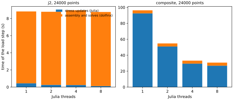
Julia's threads

06_thread_scaling.py. One load step of a cube of 24,000 points, with Julia on 1, 2, 4 and 8 threads, each run in its own process. For J2 plasticity the stress updates are 1 to 5 % of the step, which the assembly and the linear solves fill. For the composite of two viscoplastic phases they are 96 % of it, and 4 threads take 29.4 s where one takes 92.5 s (3.2 times faster), 8 threads 26.8 s; every run computes the same solution.