The quasi-elastic affine formulation

The whole page as one script

Every block of this page, in order, is scripts/material_laws/20_quasi_elastic.jl. From a clone of the repository, julia --project=docs -e 'using Pkg; Pkg.instantiate()' once, then julia scripts/material_laws/20_quasi_elastic.jl, runs it end to end.

The affine formulation for elasto-viscoplastic composites solves, at every step, a thermoelastic composite at each collocation point of a numerical inversion of the Laplace–Carson transform. Brenner et al. (2002) replace that inversion by a direct one, a single value of the transform standing for the function at a given time. The comparison composite then becomes an elastic one with an eigenstrain, in time: a "quasi-elastic" composite, solved once per step. This page states it for a matrix with inclusions and the Mori–Tanaka scheme. The example below compares it with the formulation it approximates.

The phases

Each phase is a nonlinear viscoelastic solid of Maxwell type,    , with an elastic compliance and a viscous strain rate that depends on the stress alone, such as NortonViscoplasticity.

The linearization and the direct inversion

At the time , the viscous rate is linearized about the current stress of the phase,  , and the rest of it is an eigenstrain rate that follows the actual history:

the Stieltjes convolution. In the Laplace–Carson domain the creep function    becomes  . The direct inversion takes a transform at   for the function at , which turns the convolution into a product: at   the phase is an elastic solid of compliance    with the eigenstrain . The paper shows on linear Maxwell phases that   makes the inversion exact for the creep of a single phase, and exact for a composite at the start and in the steady regime; and that      makes it exact for the relaxation, and for a constant strain rate, of a single phase of relaxation time , an average relaxation time of the phases standing for it in a composite.

The composite

The two quasi-elastic phases form a thermoelastic composite that the Mori–Tanaka scheme homogenizes as in the affine formulation, the Eshelby tensor in the isotropic part of the modulus of the matrix. The average strain of the inclusions is a fixed point: the stresses of the phases set their linearizations, which set the concentration. The eigenstrain needs only two integrals of the history of each phase, its inelastic strain and the integral of its stress, taken by the backward Euler scheme over the steps.

Scope

phases	a matrix and inclusions of Maxwell type without internal variable: NortonViscoplasticity
inversion	(creep), or built on a relaxation_time (relaxation, constant strain rate)
checks	a single phase is exact in creep and, with , in relaxation; linear Maxwell phases in creep give the elastic and the viscous Mori–Tanaka estimates at the start and in the steady regime
cost	one thermoelastic composite per iteration of a step, against one per collocation point for AffineEVPComposite

Example: creep of a two-phase composite

A matrix with 20 % of stiffer, more viscous spheres, both of Norton type of exponent 3, crept under a constant uniaxial stress:

using MeanFieldHomogenization, TensND, Plots

f = 0.2
laws = (M = NortonViscoplasticity(; E = 70e3, ν = 0.3, K = 1000.0, n = 3),
        P = NortonViscoplasticity(; E = 400e3, ν = 0.25, K = 3000.0, n = 3))
rve = RVE()
add_phase!(rve, :M, Ellipsoid(1.0), Dict(:C => TensISO{3}(1.0, 1.0)); fraction = :rest)
add_phase!(rve, :P, Ellipsoid(1.0), Dict(:C => TensISO{3}(1.0, 1.0)); fraction = f)
creep = LoadingPath(vcat(0.0, exp10.(range(-3, 1; length = 41))); σ11 = 100.0)

code	theory
QuasiElasticComposite(rve, laws)	the quasi-elastic affine formulation,
AffineEVPComposite(rve, laws; relaxation_times)	the affine formulation with the collocation inversion

p = plot(; xlabel = "time (s)", ylabel = "axial strain (%)", xscale = :log10, legend = :topleft)
for (c, label) in ((QuasiElasticComposite(rve, laws), "quasi-elastic"),
                   (AffineEVPComposite(rve, laws; relaxation_times = exp10.(range(-3, 3; length = 20))), "affine, collocation"))
    r = point_response(c, creep)
    plot!(p, r.t[2:end], r[:ε11][2:end] * 100; lw = 2, label)
end
p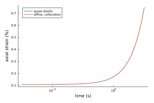

Both start from the elastic response of the Mori–Tanaka estimate and creep at nearly the same rate; the quasi-elastic formulation solves one composite per iteration instead of one per collocation point.

---

This page was generated using Literate.jl.