The affine formulation for elasto-viscoplastic composites

The whole page as one script

Every block of this page, in order, is scripts/material_laws/19_affine_evp.jl. From a clone of the repository, julia --project=docs -e 'using Pkg; Pkg.instantiate()' once, then julia scripts/material_laws/19_affine_evp.jl, runs it end to end.

The affine formulation linearizes phases whose stress is a function of the strain alone. Pierard and Doghri (2006) extend it to phases with a history: elastic, viscoplastic, and hardening with their accumulated strain. Linearized in time, such a phase is a linear viscoelastic solid with an eigenstrain, which the Laplace–Carson transform turns into a thermoelastic one, so that a linear scheme can concentrate the strain. This page states the formulation for a matrix with inclusions and the Mori–Tanaka scheme, as in the paper. The example below runs it.

The phases

Each phase (  the matrix,   the inclusions, of volume fractions ) is elasto-viscoplastic in rate form,

with its elastic compliance and an accumulated strain that hardens it, as in PerzynaViscoplasticity; a phase without hardening, such as NortonViscoplasticity, has no .

The linearization at the end of a step

At the end of a step, the rates are expanded about the current stress and accumulated strain of the phase,

, , , the derivatives of the rates in the stress and in at . Integrating the second equation and carrying into the first gives a linear viscoelastic solid. The paper applies this linear solid to the whole time axis, with an eigenstrain that makes it follow the actual inelastic rate of the phase up to and the linearized one after it. In the Laplace–Carson domain, of variable , the linear solid is a thermoelastic one,

The compliance is equation (47) of the paper. Writing the eigenstrain out, the terms in which the past enters through cancel between before and after , and what remains needs only two integrals of the history,     and    :

This is times equation (48) of the paper, which transforms the rate of the eigenstrain rather than the eigenstrain, for a history starting from rest. For a linear phase,    without , it vanishes: the phase is exactly its linear viscoelastic solid.

The comparison composite

The two thermoelastic phases, of moduli   and eigenstrains , form a composite that the Mori–Tanaka scheme homogenizes at each . With the Eshelby tensor of the inclusions, computed in the isotropic part of as the paper does after Doghri and Ouaar (2003), and   , the inclusion in the matrix strain strains as

being equation (20) of the paper and the second term the effect of the eigenstrains, the polarization of the inclusion relative to the matrix. With   ,

the same concentration as the paper's equations (17)–(19), written without the inverse of  : two identical phases are allowed, and then   and  .

Back to time

and are brought back to time by the collocation of the paper's appendix B: a function       , of transform    , matching the transform at   for the given relaxation times , with its value at   (the elastic concentration for , zero for ) and the limit of at zero, read by extrapolation from two points far below the collocation points. The average strain of the inclusions at is then

whose integral needs only the memories   . The integrals of the history are kept at the collocation points and updated step by step, a fixed amount of memory whatever the length of the history.

The step

The phases are integrated over the step at the average strains and  , which sets their linearizations and so the concentration; the strain of the inclusions it returns must be the one they were integrated at. The package iterates this fixed point by successive substitutions, as the paper does, accelerated as Anderson (1965) proposes. The macroscopic stress is the average of the stresses of the phases, the first of the two choices of the paper (its section 3.4). The consistent tangent follows by the implicit-function theorem, from the tangents of the phases and the derivative of the concentration.

Scope

phases	a matrix and inclusions of laws in rate form: PerzynaViscoplasticity, NortonViscoplasticity
scheme	Mori–Tanaka, the Eshelby tensor in the isotropic part of the matrix modulus (isotropic = false takes the whole modulus)
checks	two identical phases give the phase; elastic phases the elastic Mori–Tanaka estimate; linear Maxwell phases the linear viscoelastic one, computed in closed form, which the steps approach at the first order of their backward Euler scheme
not covered	the second moments of the strain as reference of the linearization, the macroscopic stress from the viscoelastic relation of the comparison composite (the second choice of the paper), more than two phases

Example: a particle-reinforced elasto-viscoplastic composite

A matrix holds 20 % of stiffer and stronger spherical particles, both of Perzyna type with linear hardening, pulled at a constant strain rate with free lateral faces.

using MeanFieldHomogenization, TensND, Plots

f = 0.2
matrix = PerzynaViscoplasticity(; E = 70e3, ν = 0.3, σY = 100.0, η = 1e5, m = 2.0, hardening = p -> 2e3 * p)
particles = PerzynaViscoplasticity(; E = 400e3, ν = 0.25, σY = 500.0, η = 1e6, m = 2.0, hardening = p -> 1e4 * p)
rve = RVE()
add_phase!(rve, :M, Ellipsoid(1.0), Dict(:C => TensISO{3}(1.0, 1.0)); fraction = :rest)
add_phase!(rve, :P, Ellipsoid(1.0), Dict(:C => TensISO{3}(1.0, 1.0)); fraction = f)
laws = (M = matrix, P = particles)
θ = exp10.(range(-3, 3; length = 20))                          # relaxation times of the collocation, s

code	theory
AffineEVPComposite(rve, laws; relaxation_times = θ)	the affine formulation of Pierard and Doghri, Mori–Tanaka on the comparison composite
IncrementalTangent(rve, laws)	the incremental tangent approach, the consistent tangents projected on the isotropic tensors
UniformStrain, UniformStress	the uniform-field composites

Tension

A strain rate of   up to 1 %:

pull = LoadingPath(range(0, 10; length = 41); ε11 = t -> 1e-3 * t)
p = plot(; xlabel = "axial strain (%)", ylabel = "axial stress (MPa)", legend = :bottomright)
for (c, label, ls) in ((UniformStrain(laws, (M = 1 - f, P = f)), "uniform strain", :dash),
                       (IncrementalTangent(rve, laws), "incremental tangent", :solid),
                       (AffineEVPComposite(rve, laws; relaxation_times = θ), "affine", :solid),
                       (UniformStress(laws, (M = 1 - f, P = f)), "uniform stress", :dash))
    r = point_response(c, pull)
    plot!(p, r[:ε11] * 100, r[:σ11]; lw = 2, ls, label)
end
p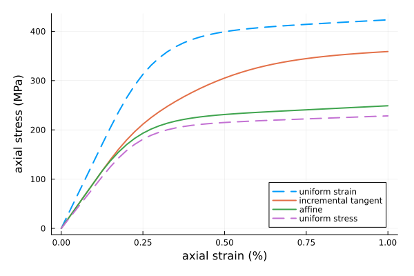

The affine estimate lies below the incremental tangent one, which Pierard and Doghri (2006) found too stiff when the tangent of a time step is used for elasto-viscoplastic phases, and between the uniform-field bounds.

Check

Two identical phases are the phase itself:

c = AffineEVPComposite(rve, (M = matrix, P = matrix); relaxation_times = θ)
point_response(c, pull)[:σ11] ≈ point_response(matrix, pull)[:σ11]

true

---

This page was generated using Literate.jl.