
CEM I 52.5 N and slag pastes, integrated in time
The same pastes
CEM I 52.5 N and slag in an isothermal calorimeter, read off the states and the bound water of the same pastes read them at the degrees of hydration the image analysis measured; the clinker kinetics page introduces the Parrott–Killoh law.
The two pages before this one take the degrees of hydration of the pastes of Gruyaert et al. (2010) as measured and compute the states they lead to. Here the degrees are not given: the pastes are integrated from the mixing, the four clinker phases dissolving under the Parrott–Killoh law, the slag glass under the Waller law, and the equilibrium solved along the way. The comparison with the article is then a test of the rate laws, and only one number is fitted to it.
The pastes, the system and the activity model are those of the two pages before, built by scripts/gruyaert2010.jl; scripts/gruyaert2010_kinetics.jl adds the slag glass as a species (glass_species), the recipe of the unreacted mix, the rate laws and the run.
1. The slag's characteristic time, from one measurement
The Waller law gives a degree of reaction that follows a sigmoid in the logarithm of time,
at the reference temperature and fineness of the law, which are 20 °C and the slag's Blaine fineness here. No parameter set for a slag is shipped: the one the package attributed to Waller (1999) is not in the thesis. The exponent n is taken from the fly-ash set of Lavergne et al. (2018), an assumption, and τ is solved from one measurement, the 72 % of slag the image analysis found at 28 months in the paste with 50 % slag.
using ChemistryLab, DynamicQuantities, OptimaSolver, Printf, Plots
include(joinpath(pkgdir(ChemistryLab), "scripts", "gruyaert2010_kinetics.jl"))

G10(table, column; where...) = only(getproperty(literature_table("Gruyaert2010", table; where...), column))
αs_measured(days, sb) = G10("hydration_degree_slag", :alpha_slag; age_days = days * u"d", slag_to_binder = sb) / 100
τ = gruyaert_slag_time()
α_waller(t) = 1 / (1 + (ustrip(us"d", τ) / t)^WALLER_PARAMS_FLY_ASH.n)
@printf("τ = %.0f days\n", ustrip(us"d", τ))
for (days, sb) in ((852, 0.5), (2, 0.85), (852, 0.85))
    @printf("slag %.2f, %3d days: law %4.2f, measured %4.2f\n", sb, days, α_waller(days), αs_measured(days, sb))
end
τ = 221 days
slag 0.50, 852 days: law 0.72, measured 0.72
slag 0.85, 2 days: law 0.04, measured 0.04
slag 0.85, 852 days: law 0.72, measured 0.39tt = 10 .^ range(-1, log10(1018); length = 200)
fig = plot(tt, α_waller.(tt); xscale = :log10, lw = 2, ylims = (0, 1), legend = :topleft,
label = @sprintf("Waller law, τ = %.0f d, n = %.1f", ustrip(us"d", τ), WALLER_PARAMS_FLY_ASH.n),
xlabel = "age (days)", ylabel = "degree of reaction of the slag", size = (720, 400),
left_margin = 5Plots.mm, bottom_margin = 5Plots.mm, title = "The slag at 20 °C")
scatter!(fig, [852], [αs_measured(852, 0.5)]; marker = :star5, ms = 8, label = "50 % slag, measured: the calibration")
scatter!(fig, [2, 852], [αs_measured(2, 0.85), αs_measured(852, 0.85)]; marker = :diamond, ms = 6,
label = "85 % slag, measured")
fig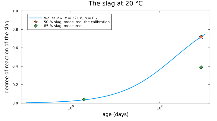
The first line is the calibration and reproduces its point. The second is a check it was not set on, the paste with 85 % slag at 2 days, and the law meets it. The third it misses by a factor of nearly two: in that paste the cement is a sixth of the binder, and the portlandite that activates a slag runs out, which a law written in the slag's own degree of reaction cannot see.
2. The cement alone
The plain paste, integrated over the 1018 days of the last bound-water measurement. The rate law of Parrott and Killoh (1984) carries its own water/cement factor (pk_wc_factor), which slows a phase once its degree passes 1.333 w/c, here 0.67.
cs0 = gruyaert_system()
plain = gruyaert_run(cs0; slag = 0.0)
clinker = ["C3S", "C2S", "C3A", "C4AF"]
day = 86400.0
αc_measured(days, sb) = G10("hydration_degree", :alpha_cement; age_days = days * u"d", slag_to_binder = sb) / 100
@printf("%d accepted steps, retcode %s\n", length(plain.sol.t), plain.sol.retcode)
for days in (2, 852)
    @printf("cement at %3d days: computed %4.2f, image analysis %4.2f\n", days,
            gruyaert_degree(plain, clinker, days * day), αc_measured(days, 0.0))
end
183 accepted steps, retcode Success
cement at 2 days: computed 0.47, image analysis 0.54
cement at 852 days: computed 0.85, image analysis 0.74Neither law reads the equilibrium partition, so the trajectory does not depend on it: the run solves it at each accepted step only to report it, with the interior point. Every number below is computed on the certified replay of the run (speciated_states).
The heat is read off the certified replay of the run (heat_release), from the unreacted mix, and compared with the reaction degree of (Gruyaert et al., 2010; Table 6) times the total heat of its Table 2.
Q_total = ustrip(us"J/g", G10("isothermal_total_heat", :heat_infinity; slag_to_binder = 0.0))
r(days) = G10("reaction_degree", :r; age_days = days * u"d", slag_to_binder = 0.0) / 100
t, Q, _ = heat_release(plain.sol, plain.kp; times = [2.0, 7.0] .* day, reference = plain.kp.initial_state)
for (days, q) in zip((2, 7), Q)
    @printf("heat at %d days: computed %5.1f J/g, measured %5.1f J/g\n", days, q / 100, r(days) * Q_total)
end
heat at 2 days: computed 246.6 J/g, measured 246.8 J/g
heat at 7 days: computed 325.4 J/g, measured 376.7 J/gNothing in this was fitted. The heat at 2 days is the measured one to 0.1 %, the degree of hydration 13 % below the image analysis; at 7 days the heat is 14 % below. At 28 months the cement is at 85 % against 74 %: the water/cement factor brings the law down from the 94 % it reaches without it, and the 74 % of Gruyaert et al. (2010) is the ultimate degree they compute for this w/c.
3. The blends
With slag the cement has more water to hydrate in, w/c = w/b / (1 − s), 1.0 for 50 % slag and 3.3 for 85 %, and the water/cement factor no longer acts.
slag_sp = gruyaert_slag_species()
cs1 = gruyaert_kinetic_system(slag_sp)
# `Any`: the type of a run is long enough that a dictionary specialized on it
# takes minutes to compile.
blends = Dict{Float64, Any}(sb => gruyaert_run(cs1; slag = sb, τ_slag = τ, slag_species = slag_sp) for sb in (0.5, 0.85))
# Not every age was measured for every paste: a dash where Table 5 has nothing.
measured(f, days, sb) = try
    @sprintf("%4.2f", f(days, sb))
catch
    "  — "
end
println("slag  days   cement: computed  measured   slag: computed  measured")
for sb in (0.5, 0.85), days in (2, 852)
    @printf("%4.2f  %4d           %4.2f      %s           %4.2f      %s\n", sb, days,
            gruyaert_degree(blends[sb], clinker, days * day), measured(αc_measured, days, sb),
            gruyaert_degree(blends[sb], ["BFS"], days * day), measured(αs_measured, days, sb))
end
slag days cement: computed measured slag: computed measured
0.50 2 0.47 — 0.04 —
0.50 852 0.94 0.94 0.72 0.72
0.85 2 0.47 0.29 0.04 0.04
0.85 852 0.94 0.91 0.72 0.39The whole runs, against the image analysis at 2 days and 28 months:
grid_days = 10 .^ range(-1, log10(1018); length = 150)
maybe(f, d, sb) = try f(d, sb) catch; NaN end
fig = plot(; xscale = :log10, ylims = (0, 1), xlabel = "age (days)", ylabel = "degree of hydration (reaction)",
           legend = :outerright, size = (900, 430), left_margin = 5Plots.mm, bottom_margin = 5Plots.mm,
           title = "w/b 0.5, 20 °C: lines computed, markers measured")
for (k, (sb, run)) in enumerate(((0.0, plain), (0.5, blends[0.5]), (0.85, blends[0.85])))
    tag = @sprintf("%d %% slag", round(Int, 100sb))
    # The laws of the two blends coincide: the paste with half slag is drawn
    # wider, under the other.
    lw = sb == 0.5 ? 5 : 2
    plot!(fig, grid_days, [gruyaert_degree(run, clinker, d * day) for d in grid_days]; lw, color = k,
          label = "cement, " * tag)
    scatter!(fig, [2, 852], [maybe(αc_measured, d, sb) for d in (2, 852)]; color = k, label = "")
    sb == 0 && continue
    plot!(fig, grid_days, [gruyaert_degree(run, ["BFS"], d * day) for d in grid_days]; lw, ls = :dash, color = k,
          label = "slag, " * tag)
    scatter!(fig, [2, 852], [maybe(αs_measured, d, sb) for d in (2, 852)]; color = k, marker = :diamond, label = "")
end
fig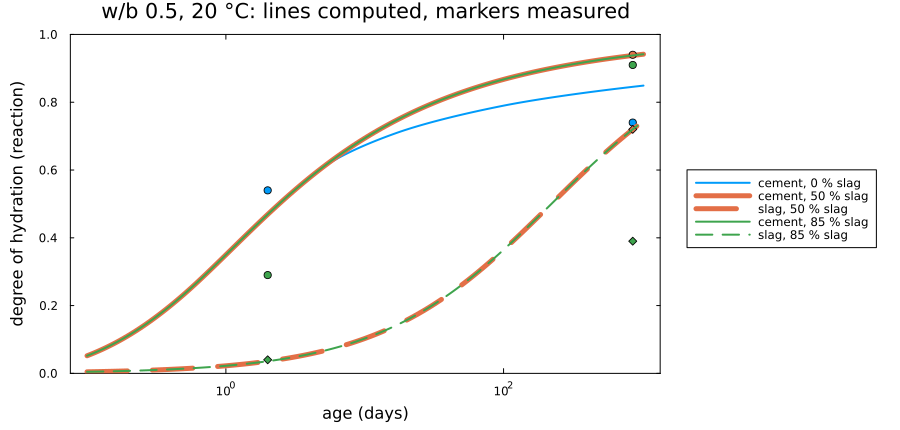
The two blends share their curves: the water/cement factor does not act on either, and the slag follows one law in both. The cement of the blends reaches 94 % at 28 months, the image analysis 94 % and 91 %: more than in the plain paste, as measured, and for the reason the factor encodes. Two numbers are missed, and they say what the laws lack. At 2 days the cement of the paste with 85 % slag is at 29 %, the law at 47 %: the Parrott–Killoh constants know nothing of the slag around the grains. And the slag of that paste stops at 39 %, where the law takes it to 72 %, for the reason of Section 1.
4. Bound water over 1018 days
The bound water of the replayed states against the thermogravimetry of (Gruyaert et al., 2010; Fig. 7), batch b, whose materials are those of the calorimetry. The calculation counts every hydrogen of the solids and the thermobalance what leaves above 105 °C once the sample has been dried, so the computed water is the larger, as on the page of the same pastes at measured degrees.
wb_measured(sb) = (tb = literature_table("Gruyaert2010", "bound_water"; batch = "b", slag_to_binder = sb);
                   (ustrip.(us"d", tb.age_days), ustrip.(tb.bound_water)))
g(q) = ustrip(uconvert(us"g", q))
println("slag   days  computed  measured  ratio")
bw_series = []
for (sb, run) in ((0.0, plain), (0.5, blends[0.5]), (0.85, blends[0.85]))
    ages, wb = wb_measured(sb)
    keep = [i for i in eachindex(ages) if ages[i] >= 1 && ages[i] <= 1019]
    states = speciated_states(run.sol, run.kp; times = ages[keep] .* day)
    computed = [g(bound_water(st)) for st in states]
    push!(bw_series, (; sb, ages = ages[keep], computed, measured = wb[keep]))
    for (k, c) in zip(keep, computed)
        @printf("%4.2f  %5.0f   %6.2f    %6.2f   %4.2f\n", sb, ages[k], c, wb[k], c / wb[k])
    end
end
slag days computed measured ratio
0.00 1 16.16 9.50 1.70
0.00 2 19.86 11.06 1.80
0.00 5 24.19 15.49 1.56
0.00 7 25.27 16.25 1.56
0.00 14 26.87 18.38 1.46
0.00 28 28.06 20.96 1.34
0.00 56 29.00 21.46 1.35
0.00 91 29.56 20.46 1.44
0.00 182 30.24 19.35 1.56
0.00 364 30.76 25.64 1.20
0.00 1018 31.36 21.43 1.46
0.50 1 8.55 5.21 1.64
0.50 4 12.91 9.32 1.39
0.50 7 14.65 10.95 1.34
0.50 14 16.63 12.97 1.28
0.50 28 19.04 17.51 1.09
0.50 56 21.75 19.44 1.12
0.50 91 23.74 17.40 1.36
0.50 186 26.36 19.96 1.32
0.50 279 27.84 17.93 1.55
0.50 1018 32.03 20.19 1.59
0.85 4 5.64 5.01 1.13
0.85 8 7.23 6.72 1.08
0.85 14 8.58 8.07 1.06
0.85 30 10.88 10.55 1.03
0.85 57 14.43 10.58 1.36
0.85 92 17.12 8.77 1.95
0.85 182 21.21 10.60 2.00
0.85 275 23.76 9.26 2.57
0.85 363 25.46 11.49 2.22fig = plot(; xscale = :log10, xlabel = "age (days)", ylabel = "bound water (g per 100 g of binder)", legend = :outerright,
size = (900, 430), left_margin = 5Plots.mm, bottom_margin = 5Plots.mm,
title = "Bound water, w/b 0.5, 20 °C: lines computed, markers measured", titlefontsize = 11)
for (k, s) in enumerate(bw_series)
tag = @sprintf("%d %% slag", round(Int, 100s.sb))
plot!(fig, s.ages, s.computed; lw = 2, color = k, marker = :circle, ms = 3, label = "computed, " * tag)
scatter!(fig, s.ages, s.measured; color = k, marker = :diamond, label = "measured, " * tag)
end
fig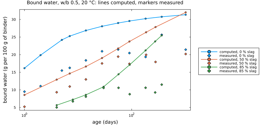
For the plain paste and the paste with 50 % slag the ratio stays between 1.1 and 1.8 over the 1018 days, the gap of definition the page at measured degrees finds at its four points. The paste with 85 % slag is different: the ratio is 1.03 to 1.13 up to a month, then grows to 2.6, the measured water holding near 10 g while the computed one keeps rising with a slag the law goes on reacting. It is the miss of Section 1, read on a second observable.
What these runs do not do
The heat of a blend. A glass has no enthalpy of formation in any database, so the heat of the blends is not computed; the calorimetry page derives the enthalpy the glass would need, and fed back here it would reproduce the measured heat by construction.
Temperature. The slag's rate carries the apparent activation energy the article fits for it at the paste's cement-to-binder ratio (its Eq. 3), and the clinker the energies of Lavergne et al. (2018); at 20 °C, the reference temperature of both laws, neither acts.
The activation of the slag by portlandite, and the early slowdown of the cement in a paste that is mostly slag: no published law of either is wired, and Sections 1 and 3 show where their absence is measured.