
Seawater flushed through a ground paste
Before this page
Seawater: a CEM I 42.5 R with limestone, titrated by the sea, for the paste in contact with increasing volumes of seawater, and the phases the sea forms in it.
De Weerdt and Justnes (2015) ground a well-hydrated paste of CEM I 42.5 R, w/c 0.4, packed 50 g of it in the thimble of a Soxhlet extractor, and dripped 100 L of seawater from the Trondheim fjord through it over six weeks, the 50 mL chamber filling and emptying some two thousand times. They measured the elements of the paste dried at 105 °C before and after the exposure (their Fig. 4) and identified its phases. This page computes the exposure as successive renewals of the pore solution by that seawater, with Cemdata18 (Lothenbach et al., 2019) and the phases of the seawater page, and compares the elements. One parameter is fitted, and the page says which.
The paste and the seawater
The paper gives the cement (Table 1), the seawater (Table 3), the mass of moist paste and its water. What it leaves open is chosen here, and each choice is stated:
the 4.1 % of limestone is part of the CaO of the oxide analysis, and is taken out of the clinker as calcite;
the clinker is 90 % reacted, the authors' estimate from the bound water, at 20 °C;
the 21 % of bound water is read per mass of ignited paste, so that the 50 g of moist paste, with 38 % of evaporable water, hold 25.6 g of cement (per mass of moist paste, they would hold 20.5 g);
the seawater of Table 3 carries more anion than cation equivalents, and its charge is closed on sodium, 1 mL weighing 1 g of water;
each filling of the chamber replaces the whole pore solution.
using ChemistryLab, DynamicQuantities, OptimaSolver, Printf, Plots
default(framestyle = :box, grid = false)
include(joinpath(pkgdir(ChemistryLab), "scripts", "seawater_flushing.jl"))

s = dj_sample()
g = dj_charge_gap()
@printf("cement in the sample %.1f g; one filling %.0f mL and the whole exposure %.3g mL per 100 g of cement\n",
        s.cement, s.filling, s.total)
@printf("seawater: cations %.3f eq/L, anions %.3f eq/L; sodium %.3f mol/L printed, %.3f to close the charge\n",
        g.cations, g.anions, g.Na_printed, g.Na_closed)
cement in the sample 25.6 g; one filling 195 mL and the whole exposure 3.9e+05 mL per 100 g of cement
seawater: cations 0.530 eq/L, anions 0.601 eq/L; sodium 0.413 mol/L printed, 0.484 to close the chargeThe paste before exposure
Before the exposure every element of the cement is in the paste, so its ratios to calcium check the reading of the cement rather than the chemistry:
path = dj_path(2000)
m = dj_measured()
println("         here     Fig. 4 (original)")
for e in (:Mg, :S, :Na, :K, :Al)
    @printf("%2s/Ca  %7.4f   %7.4f\n", e, path.initial[e] / path.initial[:Ca], m.original[e])
end
here Fig. 4 (original)
Mg/Ca 0.0390 0.0393
S/Ca 0.0348 0.0352
Na/Ca 0.0083 0.0086
K/Ca 0.0194 0.0197
Al/Ca 0.0589 0.0617The chloride of the original paste, 0.07 % of the dry sample, is not in the oxide analysis of Table 1 and is not here.
The exposure, renewal after renewal
Two thousand renewals of 195 mL of seawater per 100 g of cement, each equilibrium certified:
rows = path.rows
println("certified: ", count(r -> r.certified, rows), " of ", length(rows))
V = [r.V for r in rows]
first_with(s) = (k = findfirst(r -> get(r.solids, s, 0.0) > 1.0e-6, rows); k === nothing ? NaN : V[k])
last_with(s) = (k = findlast(r -> get(r.solids, s, 0.0) > 1.0e-6, rows); k === nothing ? NaN : V[k])
@printf("Friedel's salt present up to %.0f mL; brucite from %.0f mL; thaumasite from %.0f mL;\n",
        last_with("C4AClH10"), first_with("Brc"), first_with("thaumasite"))
@printf("portlandite gone after %.0f mL; gypsum from %.0f mL; M-S-H from %.0f mL\n",
        last_with("Portlandite"), first_with("Gp"), first_with("M15SH"))
peak(e) = V[argmax([r.elements[e] for r in rows])]
@printf("the solids hold the most chloride at %.0f mL, the most sulfur at %.0f mL, the most magnesium at %.0f mL\n",
        peak(:Cl), peak(:S), peak(:Mg))
certified: 2000 of 2000
Friedel's salt present up to 585 mL; brucite from 1366 mL; thaumasite from 781 mL;
portlandite gone after 4489 mL; gypsum from 6440 mL; M-S-H from 9173 mL
the solids hold the most chloride at 195 mL, the most sulfur at 5074 mL, the most magnesium at 16394 mLThe solids along the path, the members of each solid solution summed:
phase_label(s) = startswith(s, "CSHQ") || s in ("KSiOH", "NaSiOH") ? "C-S-H" :
    s in ("M075SH", "M15SH") ? "M-S-H" : s in ("monosulphate12", "C4AH13") ? "AFm (SO₄, OH)" :
    s in ("C3AH6", "C3FH6") ? "hydrogarnet" :
    get(Dict("Portlandite" => "portlandite", "Cal" => "calcite", "C4AClH10" => "Friedel's salt",
             "C4AsClH12" => "Kuzel's salt", "Brc" => "brucite", "Gp" => "gypsum",
             "FeOOHmic" => "iron hydroxide", "AlOHmic" => "aluminum hydroxide", "Amor-Sl" => "silica"), s, s)
grams(r) = (out = Dict{String, Float64}();
            for (s, n) in r.solids
                m = first(split(s, '#'))
                out[phase_label(m)] = get(out, phase_label(m), 0.0) + n * ustrip(us"g/mol", SW_DB[m][:M])
            end; out)
masses = [grams(r) for r in rows]
shown = sort([k for k in union(keys.(masses)...) if maximum(get(m, k, 0.0) for m in masses) > 0.5];
             by = k -> -maximum(get(m, k, 0.0) for m in masses))
fig = plot(; xscale = :log10, xlabel = "seawater (mL per 100 g of cement)", ylabel = "g per 100 g of cement",
           legend = :outerright, size = (900, 450), left_margin = 5Plots.mm, bottom_margin = 5Plots.mm,
           title = "195 mL renewals of seawater, 2000 times, 20 °C")
# Ten colors, then the same ten dashed: two neighbors in a palette are too
# alike to tell eleven curves apart.
for (j, k) in enumerate(shown)
    plot!(fig, V, [get(m, k, 0.0) for m in masses]; lw = 2, label = k,
          color = palette(:tab10)[mod1(j, 10)], ls = j > 10 ? :dash : :solid)
end
fig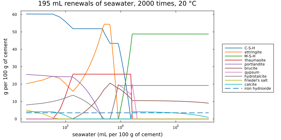
Friedel's salt, which the first renewals form, is gone by 585 mL; thaumasite forms from 781 mL and brucite from 1366 mL; the portlandite is gone after 4489 mL; gypsum forms from 6440 mL and M-S-H from 9173 mL, as the C-S-H is consumed.
And the elements the solids hold, which is what (De Weerdt and Justnes, 2015; Fig. 4) measures:
fig = plot(; xscale = :log10, yscale = :log10, ylims = (1.0e-2, 100), xlabel = "seawater (mL per 100 g of cement)",
           ylabel = "g in the solids per 100 g of cement", legend = :outerright, size = (900, 420),
           left_margin = 5Plots.mm, bottom_margin = 5Plots.mm, title = "Elements held by the solids")
for e in (:Ca, :Mg, :S, :Cl, :Al, :Na)
    plot!(fig, V, [max(r.elements[e], 1.0e-3) for r in rows]; lw = 2, label = String(e))
end
fig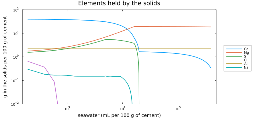
The calcium goes on leaving, and by the end of the exposure the paste holds less than 1 % of it:
plot(V, [r.retained for r in rows]; xscale = :log10, lw = 2, label = "here",
     xlabel = "seawater (mL per 100 g of cement)", ylabel = "calcium retained", legend = :topright)
hline!([m.retained]; ls = :dash, color = :black, label = "measured after 100 L")
vline!([s.total]; ls = :dot, color = :gray, label = "the exposure")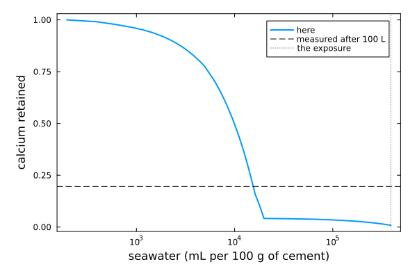
The measured sample retained a fifth of its calcium. Computed this way, the paste is a fifth of its calcium after about a twenty-fifth of the seawater that went through it.
Where the calcium retained is the measured one
The one parameter fitted here is the volume of seawater the paste is taken to have equilibrated with, read where the calcium retained is the measured one. The other ratios are then compared there, with nothing else adjusted:
x = dj_match(rows, m.retained)
@printf("volume equilibrated: %.0f mL per 100 g of cement, %.1f %% of the volume passed\n\n", x.V, 100x.V / s.total)
println("          solids   with the pore water   Fig. 4 (exposed)")
for e in (:Mg, :S, :Cl, :Na, :K, :Al)
    @printf("%2s/Ca  %8.3f   %8.3f              %8.3f\n", e, x.ratios[e], x.ratios_pw[e], m.exposed[e])
end
println("\nsolids around that point (mol per 100 g of cement):")
for (sp, n) in sort(collect(x.after); by = p -> -p[2])
    @printf("  %-14s %.4f\n", sp, n)
end
volume equilibrated: 15479 mL per 100 g of cement, 4.0 % of the volume passed
solids with the pore water Fig. 4 (exposed)
Mg/Ca 2.389 2.336 2.103
S/Ca 0.497 0.496 0.189
Cl/Ca 0.000 0.180 0.457
Na/Ca 0.000 0.103 0.210
K/Ca 0.000 0.003 0.011
Al/Ca 0.301 0.294 0.315
solids around that point (mol per 100 g of cement):
M15SH 0.2682
Brc 0.1942
Gp 0.0931
hydrotalcite 0.0433
FeOOHmic 0.0396
thaumasite 0.0264
Cal 0.0149els = (:Mg, :S, :Cl, :Na, :K, :Al)
xs = collect(eachindex(els))
w = 0.27
fig = bar(xs .- w, [x.ratios[e] for e in els]; bar_width = w, label = "solids", color = :steelblue,
xticks = (xs, ["$(e)/Ca" for e in els]), ylabel = "mass ratio to calcium", legend = :topright,
ylims = (0, 1.15 * maximum(max(x.ratios[e], m.exposed[e]) for e in els)),
size = (800, 400), left_margin = 5Plots.mm, bottom_margin = 5Plots.mm,
title = @sprintf("At %.0f mL per 100 g of cement, against Fig. 4", x.V))
bar!(fig, xs, [x.ratios_pw[e] for e in els]; bar_width = w, label = "with the pore water", color = :lightblue)
bar!(fig, xs .+ w, [m.exposed[e] for e in els]; bar_width = w, label = "measured, exposed", color = :black)
fig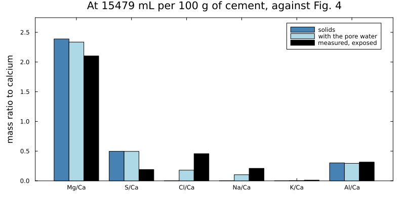
"With the pore water" adds the solutes of the 74 g of water per 100 g of cement that the moist sample held, which drying leaves in it: the paper reports halite in the dried sample.
What the comparison says
Where the calcium retained matches, the magnesium and the aluminum are near the measurement: Mg/Ca 14 % above it (11 % with the pore water), Al/Ca 4 % below. The portlandite is gone, brucite and M-S-H have formed, and gypsum is present, as the authors observe. The sulfur is two and a half times too high, the chloride and the sodium too low, and the paste here holds neither ettringite, nor C-S-H, nor a chloride AFm, all of which the authors find in the exposed sample.
What differs is not a constant of the database but the picture. Here each renewal brings the whole paste to equilibrium with the seawater it receives, so the paste moves along one path, and a state that keeps C-S-H and ettringite is a state that has not yet lost a fifth of its calcium. The authors' sample is a ground paste of grains up to a millimeter, and they find two kinds of particles in it after the exposure (Section 3): some rich in calcium, holding ettringite and a decalcified C-S-H that took up chloride, others rich in magnesium, made of M-S-H and brucite. Such a mixture lies on no single point of one path. The volume fitted, a twenty-fifth of what went through, is accordingly an apparent parameter: the share of the seawater with which the paste as a whole behaves as if it had equilibrated.
The order in which the paste takes up the elements along the path, chloride, then sulfate, then magnesium, is the order the authors' Fig. 1 shows from the inside of the concrete wall outward, from the profiles of a ten-year tidal-zone wall: chloride deepest, sulfate in between, magnesium at the surface.
The carbonate here is calcite: Cemdata18 holds aragonite, less stable, and the equilibrium does not form it. The authors identify the carbonate of the exposed paste as aragonite (Section 3).