
Solid solutions in a calculation
Before this page
Chemical Equilibrium, for a first certified solve. Why a solid solution forms, how its presence is decided and what the certificate proves are the subject of Solid solutions and Proving that an answer is the answer; this page drives a calculation and points to them.
A solid solution is declared as a candidate, and the calculation decides whether it is present, in which amount and with which composition. This tutorial follows one such calculation from end to end on the simplest gel of a cement paste: the calcium silicate hydrate formed by lime and silica in water, described by the CSHQ model of Cemdata18 (Lothenbach et al., 2019; Kulik, 2011). It declares the gel, reads which phases the equilibrium holds, explains from the output why the gel is absent or present, makes the choices that belong to the user, and reads the certificate.
1. Declaring the gel
A SolidSolutionPhase is a name, a list of end-members and a mixing model. CSHQ has six end-members in Cemdata18, four of calcium and silicon and two holding the alkalis; the alkali ones are left out here, since nothing below holds sodium or potassium. Cemdata18 mixes them ideally:
using ChemistryLab
using DynamicQuantities
using OptimaSolver
using Printf
using Plots
default(framestyle = :box, grid = false)

substances = build_species(datapath("cemdata18-thermofun.json"); verbose = false)
byname = Dict(symbol(s) => s for s in substances)

# The extended Debye-Hückel model Cemdata18 prescribes, with the ion size and
# B-dot of its KOH solutions, as on the other cement pages.
model = cemdata18_activity_model(:KOH)

CSHQ = ["CSHQ-TobH", "CSHQ-TobD", "CSHQ-JenH", "CSHQ-JenD"]
gel = SolidSolutionPhase("CSHQ", [byname[m] for m in CSHQ]; model = IdealSolidSolutionModel())

# The gel, portlandite and amorphous silica as candidates, with the aqueous
# species of their elements.
sp = speciation(substances, vcat(["Portlandite", "Amor-Sl"], CSHQ); aggregate_state = [AS_AQUEOUS])
cs = ChemicalSystem(sp, CEMDATA_PRIMARIES; solid_solutions = [gel])
The phases a database defines can also be read in one call, build_solid_solutions(datapath("solid_solutions.toml"), byname), which returns every solid solution of that file whose end-members are present, CSHQ with its six. Declaring a phase is not asserting that it forms: here the gel, the portlandite and the amorphous silica are three candidates, and the equilibrium chooses among them.
2. Which phases are present, and how much
The budget is a kilogram of water, 0.05 mol of silica and lime at a Ca/Si from 0.5 to 2.2, given as amounts of portlandite and amorphous silica; the equilibrium redistributes them. solid_solution_totals reads the gel back: the amount of each end-member and the moles of each element in the phase, whose ratios give its composition.
# A kilogram of water with `ca` mol of lime and `si` mol of silica, at equilibrium.
function lime_silica(ca, si)
    st = ChemicalState(cs)
    set_quantity!(st, "H2O@", 1.0u"kg")
    set_quantity!(st, "Portlandite", ca * u"mol")
    set_quantity!(st, "Amor-Sl", si * u"mol")
    return equilibrate_certified(st; model)
end

amount(eq, s) = ustrip(us"mol", eq.n[findfirst(x -> symbol(x) == s, cs.species)])

ratios = 0.5:0.1:2.2
gel_CaSi, gel_Si, portlandite, silica = Float64[], Float64[], Float64[], Float64[]
println("Ca/Si   solids present                    gel Ca/Si   certified")
for r in ratios
    eq, cert = lime_silica(0.05r, 0.05)
    e = solid_solution_totals(eq, "CSHQ").elements
    push!(gel_CaSi, e[:Ca] / e[:Si]); push!(gel_Si, 1000e[:Si])
    push!(portlandite, 1000amount(eq, "Portlandite")); push!(silica, 1000amount(eq, "Amor-Sl"))
    present = [k for (k, v) in (("gel", gel_Si[end]), ("portlandite", portlandite[end]),
                                ("amorphous silica", silica[end])) if v > 1.0e-6]
    @printf("%4.1f    %-33s %8.3f    %s\n", r, join(present, ", "), gel_CaSi[end], cert.optimal)
end
Ca/Si solids present gel Ca/Si certified
0.5 gel, amorphous silica 0.675 true
0.6 gel, amorphous silica 0.675 true
0.7 gel 0.703 true
0.8 gel 0.788 true
0.9 gel 0.876 true
1.0 gel 0.963 true
1.1 gel 1.048 true
1.2 gel 1.129 true
1.3 gel 1.205 true
1.4 gel 1.274 true
1.5 gel 1.338 true
1.6 gel 1.397 true
1.7 gel 1.454 true
1.8 gel 1.508 true
1.9 gel 1.561 true
2.0 gel 1.611 true
2.1 gel, portlandite 1.628 true
2.2 gel, portlandite 1.628 truep1 = plot(ratios, gel_CaSi; marker = :circle, color = :steelblue, linewidth = 2, label = "gel",
xlabel = "Ca/Si of the lime and silica", ylabel = "Ca/Si of the gel",
title = "CSHQ, portlandite, silica; 25 °C")
plot!(p1, ratios, ratios; color = :gray, linestyle = :dash, label = "lime and silica")
p2 = plot(ratios, gel_Si; marker = :circle, color = :steelblue, linewidth = 2, label = "gel (its Si)",
xlabel = "Ca/Si of the lime and silica", ylabel = "amount (mmol)",
title = "0.05 mol of silica per kg of water", legend = :right)
plot!(p2, ratios, portlandite; marker = :diamond, color = :darkorange, linewidth = 2, label = "portlandite")
plot!(p2, ratios, silica; marker = :utriangle, color = :seagreen, linewidth = 2, label = "amorphous silica")
fig = plot(p1, p2; layout = (1, 2), size = (900, 380), left_margin = 6Plots.mm, bottom_margin = 7Plots.mm)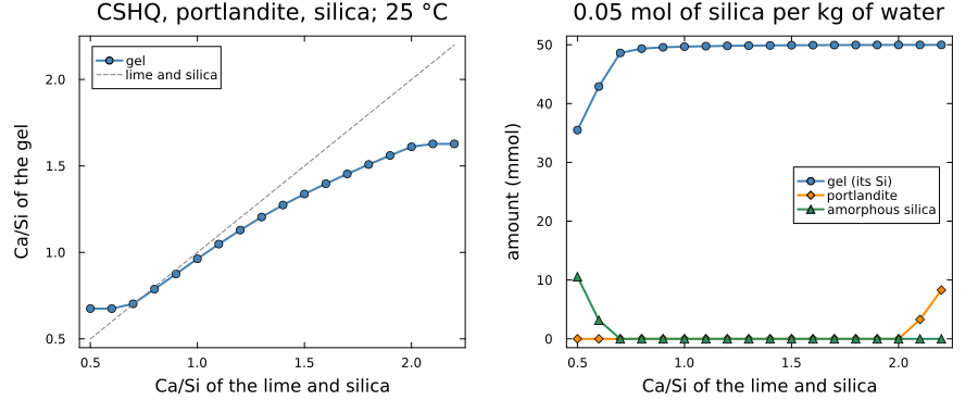
The table and the figure show three regions. Up to a Ca/Si of 0.6 the gel coexists with amorphous silica, from 0.7 to 2.0 it is the only solid, and from 2.1 it coexists with portlandite. In the middle the gel takes the composition of the whole less the calcium the solution keeps, and its Ca/Si follows the dashed line a little below it; in the two outer regions it stops, at 0.675 beside the silica and at 1.63 beside the portlandite, and the lime or the silica added beyond goes into the other solid. That plateau is the phase rule: with the solution and two solids, nothing is left free in the CaO-SiO₂-H₂O system at a given temperature and pressure (see the certifying solver). Nothing of it was told to the solver.
3. Why the gel is absent, then present
A solid solution is present when the saturation ratios its end-members would have as pure phases, saturation_indices reports for an end-member is relative to its activity log_activities. With lime and silica in equal amounts, from 0.1 to 5 mmol each per kilogram of water:
# Ωᵢ of each end-member of the gel: its saturation index, relative to its
# activity in the phase, times that activity. Both read the same log-activities,
# so this holds whether the gel is present or not.
function pure_ratios(eq)
    si = saturation_indices(eq, model)
    lna = log_activities(eq, model)
    return [exp10(si[m]) * exp(lna[m]) for m in CSHQ]
end

totals = exp10.(range(log10(1.0e-4), log10(5.0e-3); length = 15))
sum_Ω, max_Ω = Float64[], Float64[]
for c in totals
    eq, cert = lime_silica(c, c)
    Ω = pure_ratios(eq)
    push!(sum_Ω, sum(Ω)); push!(max_Ω, maximum(Ω))
end
fig = plot(1000 .* totals, sum_Ω; xscale = :log10, yscale = :log10, marker = :circle,
           label = "sum over the end-members", color = :steelblue, linewidth = 2,
           xlabel = "lime and silica (mmol of each per kg of water)",
           ylabel = "saturation ratio as a pure phase",
           title = "CSHQ at Ca/Si = 1, 25 °C", legend = :bottomright, size = (720, 420),
           left_margin = 6Plots.mm, bottom_margin = 6Plots.mm)
plot!(fig, 1000 .* totals, max_Ω; marker = :diamond, label = "largest end-member alone",
      color = :darkorange, linewidth = 2)
hline!(fig, [1.0]; color = :gray, linestyle = :dash, label = "")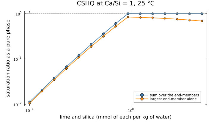
Below a threshold, near 0.9 mmol of each per kilogram of water, the sum is below one and the gel is absent, everything being in solution; from the threshold on the sum stays at one, the gel is present, and what is added beyond goes into it. The largest ratio of a single end-member stays below one throughout: none of them would precipitate alone, and their solution does. The same reading applies to a calculation in which a solid solution is unexpectedly absent: the sum says how far it is from forming.
4. The choices that belong to the user
What the end-members can hold
A solid solution can only take the compositions its end-members span, and the database says which those are. For CSHQ and for the other gel of Cemdata18 most used with blended binders, CNASH_ss (Myers et al., 2014):
CNASH = ["TobH-CNASHss", "T5C-CNASHss", "T2C-CNASHss", "5CA", "INFCA", "5CNA", "INFCNA", "INFCN"]
println("model     end-member      Ca/Si   Al/Si   Na/Si")
for (label, members) in (("CSHQ", CSHQ), ("CNASH_ss", CNASH)), m in members
    a = atoms(byname[m])
    ratio(el) = get(a, el, 0) / a[:Si]
    @printf("%-9s %-14s %6.3f  %6.3f  %6.3f\n", label, m, ratio(:Ca), ratio(:Al), ratio(:Na))
end
model end-member Ca/Si Al/Si Na/Si
CSHQ CSHQ-TobH 0.667 0.000 0.000
CSHQ CSHQ-TobD 1.250 0.000 0.000
CSHQ CSHQ-JenH 1.333 0.000 0.000
CSHQ CSHQ-JenD 2.250 0.000 0.000
CNASH_ss TobH-CNASHss 0.667 0.000 0.000
CNASH_ss T5C-CNASHss 1.000 0.000 0.000
CNASH_ss T2C-CNASHss 1.500 0.000 0.000
CNASH_ss 5CA 1.250 0.250 0.000
CNASH_ss INFCA 0.842 0.263 0.000
CNASH_ss 5CNA 1.250 0.250 0.500
CNASH_ss INFCNA 0.842 0.263 0.579
CNASH_ss INFCN 0.667 0.000 0.417CSHQ spans a Ca/Si from 0.67 to 2.25 and holds no aluminum: with it, every atom of aluminum of a paste is in another phase. CNASH_ss holds aluminum and sodium, and its Ca/Si stops at 1.5, short of the gel that sits beside portlandite in the section above. Neither limit can be removed by a setting of the solver; it is the choice of the model. Aluminum uptake by C-S-H measures what it costs on syntheses of known composition, and Aluminum in the C-S-H records two extensions that were tried and why neither is shipped.
One model of the gel at a time
CSHQ and CNASH_ss are two models of one gel, not two phases, and declaring both would share the calcium and silicon of one hydrate between two descriptions of it. The package refuses that combination:
both = [gel, SolidSolutionPhase("CNASH_ss", [byname[m] for m in CNASH])]
sp2 = speciation(substances, vcat(CSHQ, CNASH); aggregate_state = [AS_AQUEOUS])
try
    ChemicalSystem(sp2, CEMDATA_PRIMARIES; solid_solutions = both)
catch err
    println(first(split(sprint(showerror, err), ". ")), ".")
end
solid solutions "CSHQ" and "CNASH_ss" are two models of one C-S-H gel, `CSHQ` and `CNASH_ss` (data/gel_models.toml).The mixing model, and a phase that unmixes
The published model of a phase is the one to use, its end-member energies having been fitted together with its mixing model. A non-ideal model can make the phase unmix into two compositions, the miscibility gap, which a phase declared once cannot hold; Solid solutions, section 6, explains why. Whether a binary model unmixes, and where, is checked before any equilibrium: spinodal_interval returns the region where its mixing energy is concave, nothing if there is none, and common_tangent the two compositions of the gap. For a symmetric regular model, below and above the threshold of
RT = R_GAS * 298.15
for W in (1.8RT, 2.6RT)
    m = RegularSolutionModel([0.0 W; W 0.0])
    spin, ct = spinodal_interval(m, 2), common_tangent(m, 2)
    if spin === nothing
        @printf("W = %.1f RT: convex, one composition\n", W / RT)
    else
        @printf("W = %.1f RT: spinodal %.3f to %.3f, common tangent at %.3f and %.3f\n",
                W / RT, spin..., ct...)
    end
end
W = 1.8 RT: convex, one composition
W = 2.6 RT: spinodal 0.260 to 0.740, common tangent at 0.124 and 0.876The package refuses a model that unmixes when it is declared once. It is then declared with instances = 2, two coexisting compositions, or instances = :auto, which adds the second only when the certificate finds the phase wanting to split; The AFm of a CEM I and its miscibility gap runs the three declarations on the published binary.
5. Reading the certificate
equilibrate_certified returns a certificate with its answer. For the paste at a Ca/Si of 1.2:
eq, cert = lime_silica(0.06, 0.05)
@printf("optimal: %s\nelement balances: %.1e mol\nscope: %s\nstart: %s\n",
        cert.optimal, cert.balance, cert.scope, cert.route)
@printf("ionic strength %.4f mol/kg, within the range of the model: %s\n",
        cert.ionic_strength, cert.within_activity_range)
optimal: true
element balances: 7.1e-15 mol
scope: self_consistent
start: lp_start
ionic strength 0.0104 mol/kg, within the range of the model: trueoptimal says that the conditions of an equilibrium hold within their tolerances: stationarity, the element balances (the second line, in mol), and for every absent phase, the gel among them when it is absent, that it would not lower the Gibbs energy by forming. scope says what that proves. With the extended Debye-Hückel model of Cemdata18 it reads :self_consistent: the answer is a speciation consistent with its own activities, which is what that model defines, and not the minimum of one energy, which the model does not have; what the certificate proves gives the four levels and when each holds. route names the start the answer came from, here the linear program over the pure phases that the search begins with. The last line compares the ionic strength with the range the activity model states for itself: outside it, the answer is that of the model past its range, and the model rather than the solver is what limits it.
When optimal is false, the answer returned is the best one found and the certificate names what fails. The first things to check are the budget (an element no declared species can hold), a phase missing from the candidates, and the range of the activity model.
Where to go next
Solid solutions derives the mixing models, the presence test and the miscibility gap, and Proving that an answer is the answer the certifying solver and its certificate. A CEM I at equilibrium, with every solid solution declared declares every solid solution of a cement, and Aluminum uptake by C-S-H compares two models of the gel with syntheses that hold aluminum.