Validation on pore solutions over 550 days: a CEM I 42.5 N and its fly-ash blends

Before this page

Validation on early pore solutions, which does the same for the first six hours.

Deschner et al. (2012) followed the pore solution of a CEM I 42.5 N from one hour to 550 days, alone and with half of it replaced by one of two siliceous fly ashes (F1, F2), by an inert quartz powder, or by fly ash and 5 % limestone. The pastes, at a water-to-binder ratio of 0.5, were stored sealed at 23 °C. The authors analyzed potassium, sodium, calcium, silicon, aluminum and sulfur, measured the pH, and computed from each solution an effective saturation index for portlandite, gypsum, ettringite, strätlingite and monosulfate (their Table 3): log₁₀(IAP/K) divided by the number of ions the solid dissolves into, so that solids of different sizes compare.

This page computes the same indices from the same analyses, as the early pore solutions page does: each solution is only speciated, at the hydroxide measured, and nothing is equilibrated with a solid.

paste	binder (wt. %)
OPC	cement
OPC-Qz	50 cement, 50 quartz
OPC-F1, OPC-F2	50 cement, 50 fly ash
OPC-F1-L	50 cement, 45 fly ash F1, 5 limestone

Where the analyses come from

Deschner et al. (2012) print the analyses only as plots (their Figs. 13 to 16). The figures of the PDF are vector drawings, so each marker is a shape at an exact position. data/literature/Deschner2012.json holds the center of every marker, mapped to a time and a concentration through the major ticks of its panel. The ticks lie on a straight line to within 5e-4 decades, so the reading adds less than 0.2 % to the values plotted. The analyses themselves carry a standard deviation of 5 to 10 %. A concentration below the axis (0.01 mmol/L) is not plotted: aluminum in the first hours, and so no aluminous index there.

using ChemistryLab
using DynamicQuantities
using OptimaSolver
using Printf
using Plots
default(framestyle = :box, grid = false)
include(joinpath(pkgdir(ChemistryLab), "scripts", "deschner_2012.jl"))

systems = d12_systems()
# The activity model Cemdata18 prescribes, for KOH solutions: potassium is the
# main cation of every one of these solutions.
model = cemdata18_activity_model(:KOH)

1. Each analysis, speciated at its hydroxide

The analysis fixes the elements, in mmol per liter taken as mmol per kilogram of water. The authors give the free hydroxide they derived from the pH, so hydroxide is added or taken until its molality is that one. The constraint holds an activity, so the activity held is the measured molality times the activity coefficient, repeated until the coefficient no longer changes.

# `Any`: the type of a state is long enough that a dictionary specialized on it
# takes minutes to compile.
runs = Dict{Any, Any}((s, a) => d12_solution(systems.aqueous, s, a; model) for s in d12_systems_listed(), a in d12_ages())
@printf("%d solutions, certified: %d\n", length(runs), count(r -> r.certificate.optimal, values(runs)))

55 solutions, certified: 55

2. The effective saturation indices, against the paper's

labels = ["CH", "Gypsum", "Ettr", "Strätl", "MS"]
ours = Dict(k => d12_indices(r.state, systems, keys(d12_concentrations(k...)); model) for (k, r) in runs)
compared(l) = [k for k in keys(runs) if haskey(ours[k], l) && d12_published(k..., l) !== nothing]
ions = Dict(label => n for (_, (label, n)) in D12_SOLIDS)
println("index    solutions   mean difference   largest difference   the same, times the ions")
for l in labels
    d = [ours[k][l] - d12_published(k..., l) for k in compared(l)]
    @printf("%-7s  %9d   %15.3f   %18.3f   %24.2f\n", l, length(d), sum(d) / length(d), maximum(abs, d), ions[l] * maximum(abs, d))
end

index    solutions   mean difference   largest difference   the same, times the ions
CH              51             0.011                0.099                       0.30
Gypsum          51             0.011                0.068                       0.14
Ettr            37             0.009                0.030                       0.45
Strätl          37             0.007                0.028                       0.17
MS              37             0.007                0.048                       0.53

panels = map(labels) do l
    ks = compared(l)
    x = [d12_published(k..., l) for k in ks]
    y = [ours[k][l] for k in ks]
    lo, hi = extrema(vcat(x, y))
    p = plot([lo, hi], [lo, hi]; color = :gray, label = false, title = l,
             xlabel = "Deschner et al.", ylabel = "this page")
    scatter!(p, x, y; label = false, color = :steelblue, markersize = 3)
    p
end
fig = plot(panels...; layout = (1, 5), size = (1100, 260), left_margin = 6Plots.mm, bottom_margin = 8Plots.mm)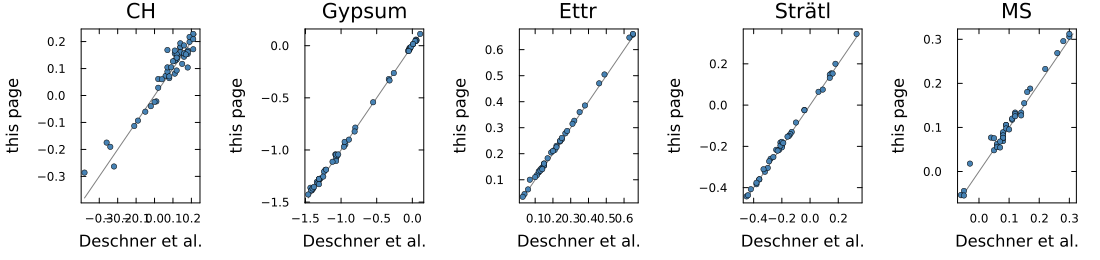

Every solution is speciated and certified. The aluminous solids agree with Deschner et al. (2012) to within 0.05: ettringite and strätlingite to 0.03, monosulfate to 0.05. Gypsum agrees to within 0.07 and portlandite to within 0.10, over five pastes and eighteen months, as the solution goes from sulfate-rich to alkaline and, in the fly-ash pastes, from saturated to undersaturated with portlandite. The mean differences are about 0.01. These indices are divided by the number of ions of the solid, from 2 for gypsum to 15 for ettringite; on the plain indices, the last column, the largest differences are 0.1 to 0.5.

Three things are left out, and each for the same reason, a value the figures do not give:

• aluminum below 0.01 mmol/L, in the first hours, and so the aluminous indices there;

• calcium at 550 days in four pastes, and so every index there but in OPC-F1;

• hemicarbonate and monocarbonate, which need the carbonate of the solution, not analyzed.

Where to go next

Validation against a measured paste follows a Portland paste through its first year, where the solids are equilibrated too.