A sorbent that appears and disappears

Before this page

Adsorption on a single site family, Chemistry that happens on a surface §10 and Standard states §4.

Everywhere else in this documentation, a surface is something that is simply there: you say how many moles of binding sites the system holds, and that number stays what you said. This page is about the case where it cannot — where the solid carrying the sites is itself dissolving, or has not precipitated yet.

It is the ordinary case in a cement paste, where the C-S-H that binds alkalis grows as the paste hydrates. It is shown here on a simpler material whose numbers are published, so that every step can be checked.

What a site is, and why its budget is a separate quantity

A mineral grain in water is not a clean cut through the crystal. The atoms at the surface have bonds that stop, and water completes them: an iron at the surface of a ferric oxide ends in a hydroxyl, written ≡FeOH. That hydroxyl is a site — one place where something can happen. It can take a proton and become positive, give one up and become negative, or hand its place to a metal ion arriving from solution.

What makes a site different from an element is that it is conserved without being matter. Turning ≡FeOH into ≡FeOH₂⁺ changes no count of iron, oxygen or hydrogen on the grain as a whole — the proton came from the water — but the number of sites is unchanged too, and nothing in the element balance says so. So the package carries a conservation row of its own for it, exactly as it does for electric charge. Surface complexation explains why that row is the right way to write it.

Why a fixed number cannot describe a dissolving sorbent

Suppose you post the site budget as a constant: 2 × 10⁻⁴ mol, say. Now add acid. The oxide dissolves; at some point half of it is gone. Half the sites went with it — but the budget still says 2 × 10⁻⁴, so the calculation keeps half a surface that no longer exists, and whatever was bound to it stays bound.

You could of course work out how much oxide survives, then re-post the budget. But how much survives depends on the surface, because the surface consumes acid too. You would need the answer before you could set up the question.

The way out is to stop posting a number and state the relation instead: one mole of this solid carries ν moles of sites, whatever amount of it there turns out to be. That relation is linear, it fits in the conservation matrix next to the element balances, and the solver then finds the amount of solid and the amount of sites together.

The material, and where its numbers come from

Hydrous ferric oxide — amorphous Fe(OH)₃, the rust-colored precipitate that forms wherever dissolved iron meets oxygen — is the reference sorbent of the field. Dzombak and Morel (1990) measured its site densities and its binding constants, and those are the numbers PHREEQC (Parkhurst and Appelo, 2013) ships to this day.

Two numbers define the surface:

• 0.2 mol of weak sites per mole of Fe(OH)₃. That is ν. (There is a second, much rarer family of "strong" sites at 0.005 mol/mol; leaving it out changes nothing about what this page shows, and the two-family case is in Two families of sites, and a metal between them.)

• log K = 7.29 and −8.93 for taking up and giving up a proton.

and one more for the metal: log K = −3.50 for ≡FeOH + Mn²⁺ ⇌ ≡FeOMn⁺ + H⁺. Manganese is chosen because it binds firmly enough that the release is visible, and because the database used here carries its aqueous chemistry.

using ChemistryLab, DynamicQuantities, SciMLBase, OptimaSolver, LinearAlgebra

const RT = R_GAS * 298.15
lnK(logK) = -RT * log(10.0^logK)         # ΔrG° = −RT ln K
energy(v) = SymbolicFunc(v * u"J/mol")

# Dzombak and Morel's weak sites per mole of iron, and PHREEQC's constants,
# read from the copy of phreeqc.dat that the test oracles use.
ν = literature_value("DzombakMorel1990", "weak_sites_per_mol_Fe")
dat = read_sorption_model(datapath("phreeqc.dat"))
log_k(product) = only(reactions_involving(dat, product)).log_K.value
logK_prot, logK_depr, logK_Mn = log_k("Hfo_wOH2+"), log_k("Hfo_wO-"), log_k("Hfo_wOMn+")

The aqueous side

Everything that is not the surface comes from a database the package ships — PSI/Nagra here, because it is the one that carries amorphous ferric hydroxide as a solid. See Where the numbers come from.

subs = build_species(datapath("psinagra-12-07-thermofun.json"); verbose = false)
db = Dict(symbol(s) => s for s in subs)
host = db["Fe(OH)3(am)"]

# Iron in one oxidation state only: there is no reductant here, so the ferrous
# species would be an unused half of a redox couple. Carbonate, sulfate and
# fluoride are left out for the same reason — nothing in the recipe supplies
# them.
aqueous = speciation(
    subs, ["Fe(OH)3(am)", "Cl-", "Mn+2"];
    aggregate_state = [AS_AQUEOUS],
    exclude_species = split(
        "H2@ O2@ Fe+2 FeOH+ FeO+ FeCl+ Cls ClO4- " *
            "MnSeO4@ MnSeO3w2(cr) Mn(CO3)@ Mn(HCO3)+ MnF+ Mn(SO4)@"
    ),
)
symbol.(aqueous)

19-element Vector{String}:
 "H2O@"
 "Fe2(OH)2+4"
 "Fe3(OH)4+5"
 "FeCl3@"
 "MnCl2@"
 "MnCl3-"
 "FeCl2+"
 "Cl-"
 "H+"
 "Mn+2"
 "FeO2-"
 "FeOH+2"
 "FeO2H@"
 "MnOH+"
 "OH-"
 "Fe+3"
 "FeCl+2"
 "MnCl+"
 "Fe(OH)3(am)"

The surface species

A surface species is an ordinary species. What marks it is its aggregate state and the site symbol in its formula — Xw here — which is what puts it in the site balance.

surface(sym, g) = (
    s = Species(sym; aggregate_state = AS_SURFACE, class = SC_SURFCOMPLEX);
    s[:ΔₐG⁰] = energy(g); s
)

The energy of the free site

The free site needs a standard energy, and with a fixed site budget any value would do: every surface reaction has a site on both sides, so the value cancels, and the package measures that invariance as part of its test suite.

With a budget that follows its host the value no longer cancels, and it has to be zero. The reason is that ≡FeOH is made of the host itself: the database formula Fe(OH)₃ already contains the hydroxyls that the surface exposes, and the database energy of the solid is the energy of the whole grain, surface included. The package therefore counts the free sites as part of the host, so that a grain whose sites are all free has exactly the composition and the energy of the database formula, which holds only if the free site itself costs nothing. Giving it the energy of the oxygen and hydrogen it carries would count that energy a second time. Every other surface species is then written relative to the free site, through its reaction constant:

G(s) = ustrip(us"J/mol", s[:ΔₐG⁰](T = 298.15u"K", P = 1.0e5u"Pa"; unit = true))

free = surface("XwOH", 0.0)                     # part of the host: zero
prot = surface("XwOH2+", lnK(logK_prot))        # ≡FeOH + H⁺ = ≡FeOH₂⁺
depr = surface("XwO-", lnK(logK_depr))          # ≡FeOH = ≡FeO⁻ + H⁺
# The manganese complex carries the aqueous manganese's own energy, because
# ≡FeOH + Mn²⁺ = ≡FeOMn⁺ + H⁺ puts it in the balance.
mn = surface("XwOMn+", lnK(logK_Mn) + G(db["Mn+2"]))
atoms(free)

OrderedCollections.OrderedDict{Symbol, Int64} with 3 entries:
  :Xw => 1
  :O  => 1
  :H  => 1

Declaring the coupling

Three pieces: the support says what carries the sites and that they follow it; the capacity says how many per unit of it; the family gathers the species.

M = ustrip(us"kg/mol", host[:M])               # kg per mole of Fe(OH)₃

support = SurfaceSupport(
    "hydrous ferric oxide", "Fe(OH)3(am)", FixedSurfaceArea(1.0);
    coupling = SITES_FOLLOW_HOST,
)
family = SiteFamily(
    "Xw", free, [prot, depr, mn];
    capacity = MassSiteDensity(ν / M),         # mol of sites per kg of host
    support,
)
ChemistryLab.sites_per_host(family, M)         # back to ν, by the same arithmetic

0.2

Naming a host does not couple anything by itself — a rate law has named one since long before, to know what amount it scales with. The coupling is asked for, with coupling = SITES_FOLLOW_HOST.

The capacity has to be one that is proportional to how much host there is, which is why it is given per unit mass. The package does not take that on trust: it evaluates the capacity at two host amounts and checks that the budget scales with them. A capacity posted as a total number of moles is refused, because a total is not a relation.

The system

The components are the ones the aqueous side needs, plus the free site, which carries the site balance:

cs = ChemicalSystem(
    AbstractSpecies[vcat(aqueous, [free, prot, depr, mn])...],
    AbstractSpecies[db["H2O@"], db["H+"], db["Fe+3"], db["Cl-"], db["Mn+2"], free];
    site_families = [family],
)
symbol.(cs.SM.primaries)

6-element Vector{String}:
 "H2O@"
 "H+"
 "Fe+3"
 "Cl-"
 "Mn+2"
 "XwOH"

A bare site component, Species("Xw+"), may be declared in place of the free site and gives the same answer; the test suite checks that the two agree.

The coupling can be checked before anything is solved. This reads, in log units of solubility, how much the energy of the free site moves the host:

host_coupling_bias(cs)

OrderedCollections.OrderedDict{String, Float64} with 1 entry:
  "Xw" => 0.0

Zero, since the free site sits at zero. Had it been given the energy of the matter it carries, μ°(H₂O) − μ°(H⁺) = −237.2 kJ/mol, the same call would read 8.3, and a family worth more than 0.05 log units is refused at construction with the value to use in the message.

The starting state

One kilogram of water, one millimole of the oxide, a tenth of a millimole of manganese, and enough chloride to balance it.

state = ChemicalState(cs)
set_quantity!(state, "H2O@", 1.0u"kg")        # `set_quantity!` converts
set_quantity!(state, "Fe(OH)3(am)", 1.0e-3u"mol")
set_quantity!(state, "Mn+2", 1.0e-4u"mol")
set_quantity!(state, "Cl-", 2.0e-4u"mol")

# Derive the free-site amount from the declaration rather than typing it: the
# state and the capacity then say the same thing by construction.
state = host_consistent_state(state)
site_budget_residual(state)

OrderedCollections.OrderedDict{String, Float64} with 1 entry:
  "Xw" => 0.0

That residual is the difference between the sites the state carries and the sites the capacity declares. Zero means they agree. If you set the amounts by hand and they disagree, check_site_budget turns it into an error rather than a quietly different calculation.

Dissolving the sorbent

The experiment is a titration: add hydrochloric acid, in steps counted as moles per mole of Fe(OH)₃. Three moles is the stoichiometric amount to dissolve it all, and rather more than that is needed in practice, because the surface and the dissolved iron both take a share.

A = conservation_matrix(cs)                    # the coupled matrix, not SM.A
b0 = A * Float64[ustrip(us"mol", x) for x in state.n]
prim = string.(symbol.(cs.SM.primaries))
iH, iCl = findfirst(==("H+"), prim), findfirst(==("Cl-"), prim)
idx = Dict(s => i for (i, s) in enumerate(symbol.(cs.species)))
model = DaviesActivityModel()

acid = [0.0, 0.05, 0.1, 0.2, 0.35, 0.5, 0.75, 1.0, 2.0, 3.0, 4.0, 4.5]

function titrate(x)
    b = copy(b0)
    b[iH] += x * 1.0e-3                        # HCl: a proton and a chloride
    b[iCl] += x * 1.0e-3
    eq, cert = equilibrate_certified(state; model = model, b = b)
    n = Float64[ustrip(us"mol", v) for v in eq.n]
    sites = sum(n[idx[s]] for s in ("XwOH", "XwOH2+", "XwO-", "XwOMn+"))
    return (
        eq = eq, optimal = cert.optimal,
        oxide = n[idx["Fe(OH)3(am)"]], sites = sites,
        bound = n[idx["XwOMn+"]] / 1.0e-4, pH = pH(eq, model),
    )
end

runs = titrate.(acid)
all(r -> r.optimal, runs)                      # every point is a certified minimum

true

using Printf
println(" HCl/Fe   Fe(OH)₃ mol   sites mol    sites/Fe(OH)₃   Mn bound %    pH")
for (x, r) in zip(acid, runs)
    @printf(
        "%6.2f   %10.3e   %10.3e   %12.6f   %9.2f   %6.3f\n",
        x, r.oxide, r.sites, r.sites / r.oxide, 100r.bound, r.pH
    )
end

 HCl/Fe   Fe(OH)₃ mol   sites mol    sites/Fe(OH)₃   Mn bound %    pH
  0.00    1.000e-03    2.000e-04       0.200000       48.97    7.538
  0.05    1.000e-03    2.000e-04       0.200000       31.75    7.284
  0.10    1.000e-03    2.000e-04       0.200000       16.80    7.030
  0.20    1.000e-03    2.000e-04       0.200000        0.03    5.499
  0.35    9.970e-04    1.994e-04       0.200000        0.00    3.851
  0.50    9.897e-04    1.979e-04       0.200000        0.00    3.564
  0.75    9.703e-04    1.941e-04       0.200000        0.00    3.322
  1.00    9.430e-04    1.886e-04       0.200000        0.00    3.178
  2.00    7.762e-04    1.552e-04       0.200000        0.00    2.894
  3.00    5.463e-04    1.093e-04       0.200000        0.00    2.761
  4.00    2.763e-04    5.527e-05       0.200000        0.00    2.681
  4.50    1.307e-04    2.614e-05       0.200000        0.00    2.651

Two different things happen, in that order, and telling them apart is the point of the page.

Up to about 0.2 mol of acid per mole of oxide, nothing dissolves. The oxide column does not move and neither does the site column. What the acid does is protonate the surface, and in doing so it takes the manganese back off it: bound manganese falls from half of the inventory to essentially none while the sorbent is still entirely present. A fixed site budget describes this perfectly well.

Past that, the oxide goes, and the sites go with it. The two columns fall together, and the ratio in the middle column stays at ν to six decimals all the way down — that is the relation being enforced, not fitted.

using Plots

p = plot(
    layout = (2, 1), size = (700, 620), link = :x,
    left_margin = 5Plots.mm, bottom_margin = 4Plots.mm,
)
plot!(
    p[1], acid, [r.oxide for r in runs] .* 1e3;
    label = "Fe(OH)₃ present", color = :firebrick, linewidth = 2, marker = :circle,
    ylabel = "mmol", title = "The sorbent, and the sites it carries",
)
plot!(
    p[1], acid, [r.sites for r in runs] .* 1e3 ./ ν;
    label = "sites ÷ ν  (should lie on top)", color = :black,
    linewidth = 2, linestyle = :dash,
)
plot!(
    p[2], acid, [100r.bound for r in runs];
    label = "manganese bound", color = :steelblue, linewidth = 2, marker = :circle,
    xlabel = "mol HCl per mol Fe(OH)₃", ylabel = "% of the manganese",
    legend = :topright,
)
plot!(twinx(p[2]), acid, [r.pH for r in runs];
      label = "pH", color = :seagreen, linewidth = 2, linestyle = :dot,
      ylabel = "pH", legend = :right)
p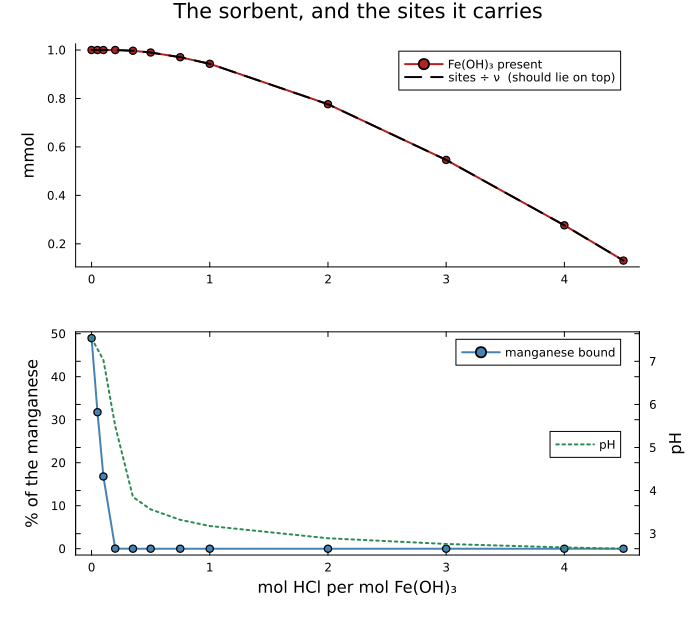

The dashed line is the site total divided by ν. It lies on the solid one because the constraint says it must; if it ever did not, the calculation would not be the one that was declared.

The three things worth checking afterwards

A solve that converges, an answer that is physically admissible and a certified minimum are three different statements. Here they are separately.

worst_ratio = maximum(abs(r.sites / r.oxide / ν - 1) for r in runs)

1.5543122344752192e-15

The relation holds. The site total is ν times the host amount, everywhere, to that relative accuracy.

element(n, e) = sum(
    n[i] * Float64(get(atoms(cs.species[i]), e, 0)) for i in eachindex(n)
)
n0 = Float64[ustrip(us"mol", x) for x in state.n]
worst_element = maximum(
    abs(element(Float64[ustrip(us"mol", v) for v in r.eq.n], e) - element(n0, e)) /
        element(n0, e) for e in (:Fe, :Mn), r in runs
)

8.131516293641283e-15

The elements are conserved. Iron and manganese are counted from the species' own formulas, which checks the matrix independently; they can be, because the sites carry neither. Oxygen and hydrogen cannot be counted that way, since the free sites are part of the host and the host's formula already includes their atoms: the coupled matrix counts every atom once, and A * n stays at its starting value.

z = [Float64(charge(s)) for s in cs.species]
worst_charge = maximum(abs(sum(z .* Float64[ustrip(us"mol", v) for v in r.eq.n])) for r in runs)

2.0826135150943694e-17

Charge is conserved, the solution and the surface together, while the host dissolves: the free sites that leave with it carry no charge.

worst_si = maximum(
    abs(saturation_indices(r.eq, model)["Fe(OH)3(am)"])
        for r in runs if r.oxide > 1.0e-9
)

2.4686783143764146e-14

Every phase that is present sits at log SI = 0. That is not a coincidence to be admired: it is the definition of being at equilibrium with the solution, and an index that disagreed with it would be a diagnostic that lies.

The same coupling in PHREEQC

PHREEQC has been able to tie a surface to a mineral since version 2, written

Hfo_wOH   Fe(OH)3(a)   equilibrium_phase   0.2

which reads exactly as SITES_FOLLOW_HOST does here. The generator test/reference/phreeqc_evolving_surface.py titrates a sorbent to exhaustion with it, and the two codes agree on the coupling law to 2 × 10⁻¹⁰ over five partially dissolved states.

The two codes do not run the same surface model, which matters before comparing anything else. In PHREEQC the site totals scale with the phase amount, and the phase's solubility is that of its database record. This package counts the free sites as part of the host, so the host's stability includes the energy of its surface, and a surface that binds protons or metals changes how soluble the host is. The two therefore agree on the ratio of sites to phase, and are expected to differ on how much of the phase dissolves.

What this page does not cover

• The sorbent exhausted. Past about five moles of acid per mole of oxide the solid is gone, its whole family sits at the solver's floor, and the solve stops certifying. The sweep above stops before that on purpose; a surface with no host is a system to describe differently, not a limit to take.

• A sorbent that appears. Everything here runs backwards as well — the same declaration describes a phase precipitating and bringing its sites with it — but the case that matters, a C-S-H forming as a paste hydrates, needs site densities for the C-S-H, for which no published value is available. That is a missing measurement, not a missing feature.

• Electrostatics. The surface here has a charge and no potential; see A charged surface, screened.

• The energy of the host's surface. Counting the free sites as part of the host, at zero energy, follows Kulik (2002), for whom the surface groups of a sorbent belong to it. It assumes that the database energy of the solid is that of its uncomplexed surface, which the measurements behind a database do not state.

See also

• Surface areas — the syntax of a coupled family.

• Surface complexation — why a site balance is a conservation row, and how Langmuir falls out of it.

• Two families of sites, and a metal between them — the same oxide with a fixed budget, against PHREEQC.