
A slow surface: sorption at a rate
Before this page
A slow surface and What a rate law may be for the theory; Adsorption on a single site family for the syntax of a surface.
A site family is solved at equilibrium unless a kinetic reaction controls one of its members. This page builds the smallest slow surface, checks it against its closed form, sets it beside a fast family, and shows what dissipation says of a law that is not tied to the equilibrium constant.
The rate constant of this page is not a measurement
The equilibrium constant below is published. The rate constant is not: the papers cited in the theory report equilibrium within milliseconds on oxide surfaces, and a slow uptake as an apparent effect of transport. The value used here, k = 10 s⁻¹, is chosen so that the relaxation takes about a quarter of an hour and can be followed. The page shows how the model behaves, not how this surface does.
The surface and the solution
One family of sites, the strong sites of hydrous ferric oxide in the model of Dzombak and Morel (1990), taking calcium:
The constant is read from the copy of phreeqc.dat the test oracles use (Parkhurst and Appelo, 2013). The family is kept to its free site and this one complex, and without a surface potential: it is not the full model of Dzombak and Morel, which also protonates and deprotonates the site and charges the surface.
using ChemistryLab, DynamicQuantities, OptimaSolver, OrderedCollections, OrdinaryDiffEq, Printf, Plots
default(framestyle = :box, grid = false)

const RT = R_GAS * 298.15
g0(v) = SymbolicFunc(v * u"J/mol")

dat = read_sorption_model(datapath("phreeqc.dat"))
logK = only(reactions_involving(dat, "Hfo_sOHCa+2")).log_K.value

db = Dict(symbol(s) => s for s in
          build_species(datapath("slop98-inorganic-thermofun.json"); verbose = false))
h2o, hp, oh, ca = db["H2O@"], db["H+"], db["OH-"], db["Ca+2"]
G_Ca = ustrip(us"J/mol", ca[:ΔₐG⁰](T = 298.15u"K", P = 1.0e5u"Pa"; unit = true))

function site(sym, g)
    s = Species(sym; aggregate_state = AS_SURFACE, class = SC_SURFCOMPLEX)
    s[:ΔₐG⁰] = g0(g)
    return s
end
# ΔrG° = G(complex) − G(free site) − G(Ca+2) = −RT ln K, with G(free site) = 0
free  = site("XsOH", 0.0)
bound = site("XsOHCa+2", -RT * log(10.0^logK) + G_Ca)
logK4.97The parameters of the run, all defined here:
N_sites = 1.0e-7          # mol of sites, a thousandth of the calcium
n_Ca    = 1.0e-4          # mol of Ca(OH)2 dissolved in one kilogram of water
k       = 10.0            # s⁻¹, illustrative (see the warning above)
t_end = 2.0e4 # s, some twenty relaxation timessupport = SurfaceSupport("hydrous ferric oxide, strong sites", nothing, FixedSurfaceArea(1.0))
family = SiteFamily("Hfo_s", free, [bound];
capacity = TotalSiteAmount(N_sites * u"mol"), support)
cs = ChemicalSystem([h2o, hp, oh, ca, free, bound], [h2o, hp, ca, free];
site_families = [family])
idx(s) = findfirst(==(s), symbol.(cs.species))
n0 = Any[fill(0.0u"mol", length(cs.species))...]
n0[idx("H2O@")] = ustrip(us"mol", 1.0u"kg" / h2o[:M]) * u"mol"
n0[idx("Ca+2")] = n_Ca * u"mol"
n0[idx("OH-")] = 2n_Ca * u"mol"
n0[idx("XsOH")] = N_sites * u"mol"
state0 = ChemicalState(cs, n0)A slow family
The reaction is written with the free site first, which makes it the species the reaction controls. sorption_rate gives it the elementary law
rxn = Reaction(OrderedDict(free => 1, ca => 1), OrderedDict(bound => 1);
               symbol = "Ca on Hfo_s", equal_sign = '→')
kr  = KineticReaction(cs, rxn, sorption_rate(k, cs, rxn))

solver = EquilibriumSolver(cs, DiluteSolutionModel(), OptimaOptimizer())
kp  = KineticsProblem(cs, [kr], state0, (0.0, t_end); equilibrium_solver = solver)
ts  = collect(range(0.0, t_end; length = 81))
ks  = KineticsSolver(; ode_solver = Rodas5P(), reltol = 1.0e-10, abstol = 1.0e-20, saveat = ts)
sol = integrate(kp, ks)
states = speciated_states(sol, kp)
symbol.(cs.species[kp.idx_kinetic])      # the kinetic side: the whole family
2-element Vector{String}:
"XsOH"
"XsOHCa+2"With a thousand times more calcium than sites, the solution barely moves, and the occupied amount follows the closed form of the theory page,
a_Ca = exp(log_activities(states[1], DiluteSolutionModel())["Ca+2"])
λ    = k * (a_Ca + 10.0^-logK)
n_eq = k * N_sites * a_Ca / λ
bound_run    = [ustrip(us"mol", s.n[idx("XsOHCa+2")]) for s in states]
bound_closed = [n_eq * (1 - exp(-λ * t)) for t in ts]
@printf("λ = %.3e s⁻¹, n_eq/N = %.4f, largest gap = %.1e of the site budget\n",
        λ, n_eq / N_sites, maximum(abs.(bound_run .- bound_closed)) / N_sites)
λ = 1.107e-03 s⁻¹, n_eq/N = 0.9032, largest gap = 1.6e-04 of the site budgetplot(ts ./ 60, bound_run ./ N_sites; label = "integrated", lw = 2,
xlabel = "time (min)", ylabel = "fraction of sites holding Ca")
plot!(ts ./ 60, bound_closed ./ N_sites; label = "closed form", ls = :dash, lw = 2)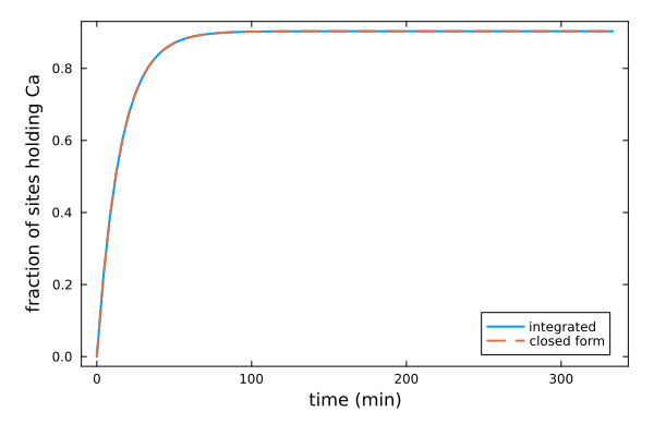
Beside a fast family
A second family with the same constant, Hfo_f, on a support of its own, that no reaction controls: it stays on the equilibrium side and follows the solution at every instant, while the slow one lags.
free_f  = site("XfOH", 0.0)
bound_f = site("XfOHCa+2", -RT * log(10.0^logK) + G_Ca)
fast = SiteFamily("Hfo_f", free_f, [bound_f]; capacity = TotalSiteAmount(N_sites * u"mol"),
                  support = SurfaceSupport("fast sites", nothing, FixedSurfaceArea(1.0)))
cs2 = ChemicalSystem([h2o, hp, oh, ca, free, bound, free_f, bound_f],
                     [h2o, hp, ca, free, free_f]; site_families = [family, fast])
idx2(s) = findfirst(==(s), symbol.(cs2.species))
n2 = Any[fill(0.0u"mol", length(cs2.species))...]
n2[idx2("H2O@")] = n0[idx("H2O@")]
n2[idx2("Ca+2")] = n_Ca * u"mol"
n2[idx2("OH-")]  = 2n_Ca * u"mol"
n2[idx2("XsOH")] = N_sites * u"mol"
n2[idx2("XfOH")] = N_sites * u"mol"
rxn2 = Reaction(OrderedDict(cs2.species[idx2("XsOH")] => 1, cs2.species[idx2("Ca+2")] => 1),
                OrderedDict(cs2.species[idx2("XsOHCa+2")] => 1); symbol = "Ca on Hfo_s", equal_sign = '→')
kp2 = KineticsProblem(cs2, [KineticReaction(cs2, rxn2, sorption_rate(k, cs2, rxn2))],
                      ChemicalState(cs2, n2), (0.0, t_end);
                      equilibrium_solver = EquilibriumSolver(cs2, DiluteSolutionModel(), OptimaOptimizer()))
sol2 = integrate(kp2, ks)
states2 = speciated_states(sol2, kp2)
slow_frac = [ustrip(us"mol", s.n[idx2("XsOHCa+2")]) / N_sites for s in states2]
fast_frac = [ustrip(us"mol", s.n[idx2("XfOHCa+2")]) / N_sites for s in states2]
plot(ts ./ 60, fast_frac; label = "fast family", lw = 2,
     xlabel = "time (min)", ylabel = "fraction of sites holding Ca")
plot!(ts ./ 60, slow_frac; label = "slow family", lw = 2)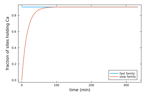
A law that ignores the database
The same mass action, with a backward constant a tenth of what the equilibrium constant gives: dissipation lists those instants.
K = 10.0^logK
bad = KineticReaction(cs, rxn,
    (T, P, t, n, lna, n0) -> k * n["XsOH"] * exp(lna["Ca+2"]) - k / (10K) * n["XsOHCa+2"])
kp_bad  = KineticsProblem(cs, [bad], state0, (0.0, t_end); equilibrium_solver = solver)
sol_bad = integrate(kp_bad, ks)
d_good = dissipation(sol, kp)
d_bad  = dissipation(sol_bad, kp_bad)
@printf("consistent law: %d violations; inconsistent law: %d violations\n",
        length(d_good.violations), length(d_bad.violations))
@printf("ln Ω at the end: consistent %.1e, inconsistent %.4f (ln 10 = %.4f)\n",
        -d_good.affinity[end, 1] / RT, -d_bad.affinity[end, 1] / RT, log(10))
consistent law: 0 violations; inconsistent law: 45 violations
ln Ω at the end: consistent -2.5e-09, inconsistent 2.3026 (ln 10 = 2.3026)lnΩ(d) = -d.affinity[:, 1] ./ RT
on = ts .> 0 # at t = 0 no site is occupied and ln Ω is unbounded
against = [findfirst(==(v.time), ts) for v in d_bad.violations]
plot(ts[on] ./ 60, lnΩ(d_good)[on]; label = "consistent law", lw = 2,
xlabel = "time (min)", ylabel = "ln Ω", ylims = (-4, 3), legend = :bottomright)
plot!(ts[on] ./ 60, lnΩ(d_bad)[on]; label = "backward constant ÷ 10", lw = 2)
scatter!(ts[against] ./ 60, lnΩ(d_bad)[against]; label = "rate against the affinity", ms = 3)
hline!([0.0, log(10)]; color = :black, ls = :dash, label = nothing)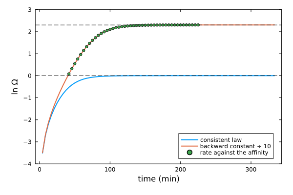
Along the consistent law
On a host that dissolves
The sites may belong to a solid that dissolves under its own rate law, their budget then following the solid's amount (A slow surface). Sites that vanish take every state in proportion to its amount and return what it held to the solution. The free site must be bare, ≡Xs, and the states written relative to it. The constants below are illustrative, like the rate constant above: the sites of portlandite, at a density of 10⁻⁵ mol/m² on 10⁵ m²/kg, binding calcium as
G(s) = ustrip(us"J/mol", s[:ΔₐG⁰](T = 298.15u"K", P = 1.0e5u"Pa"; unit = true))
portlandite = only(filter(s -> symbol(s) == "Portlandite",
                          build_species(datapath("cemdata18-thermofun.json"); verbose = false)))
xs, xsca = site("Xs", 0.0), site("XsOHCa+", -RT * log(10.0^-9.2) + G(h2o) + G_Ca)
on_host = SiteFamily("Xs", xs, [xsca];
    capacity = AreaSiteDensity(1.0e-5u"mol/m^2"),
    support = SurfaceSupport("portlandite", "Portlandite", BETSurfaceArea(1.0e5u"m^2/kg");
                             coupling = SITES_FOLLOW_HOST))
cs_h = ChemicalSystem([h2o, hp, oh, ca, portlandite, xs, xsca], [h2o, hp, ca, xs];
                      site_families = [on_host])
ih(s) = findfirst(==(s), symbol.(cs_h.species))
st_h = ChemicalState(cs_h)
set_quantity!(st_h, "H2O@", 1.0u"kg" / h2o[:M])
set_quantity!(st_h, "Portlandite", 1.0e-3u"mol")
set_quantity!(st_h, "Ca+2", n_Ca * u"mol")
set_quantity!(st_h, "OH-", 2n_Ca * u"mol")
st_h = host_consistent_state(st_h)          # the free sites the host declares

k_d = 2.0e-4                                 # s⁻¹, the solid's own rate constant
dissolve = Reaction(OrderedDict(portlandite => 1), OrderedDict(ca => 1, oh => 2);
                    symbol = "portlandite", equal_sign = '→')
st_d = Float64[get(Dict("Portlandite" => -1.0, "Ca+2" => 1.0, "OH-" => 2.0), symbol(s), 0.0)
               for s in cs_h.species]
kr_d = KineticReaction(dissolve, (T, P, t, n, lna, n0) -> k_d * n["Portlandite"], ih("Portlandite"), st_d)
bind = Reaction(OrderedDict(xs => 1, ca => 1, h2o => 1), OrderedDict(xsca => 1, hp => 1);
                symbol = "Ca on Xs", equal_sign = '→')
kr_b = KineticReaction(cs_h, bind, sorption_rate(0.05, cs_h, bind))

ts_h = collect(range(0.0, 1.5e4; length = 61))
kp_h = KineticsProblem(cs_h, [kr_d, kr_b], st_h, (0.0, ts_h[end]);
                       equilibrium_solver = EquilibriumSolver(cs_h, DiluteSolutionModel(), OptimaOptimizer()))
states_h = speciated_states(integrate(kp_h, KineticsSolver(; ode_solver = Rodas5P(), reltol = 1.0e-10,
                                                         abstol = 1.0e-20, saveat = ts_h)), kp_h)
m(s, x) = ustrip(us"mol", s.n[ih(x)])
host  = [m(s, "Portlandite") for s in states_h]
sites = [m(s, "Xs") + m(s, "XsOHCa+") for s in states_h]
calcium(s) = m(s, "Portlandite") + m(s, "Ca+2") + m(s, "XsOHCa+")
@printf("sites / (ν n_host) − 1: %.1e; calcium drift: %.1e mol\n",
        maximum(abs.(sites ./ (sites[1] .* host ./ host[1]) .- 1)),
        maximum(abs(calcium(s) - calcium(st_h)) for s in states_h))
sites / (ν n_host) − 1: 1.3e-14; calcium drift: 1.7e-17 molThe sites follow the solid exactly, and the calcium they held is back in the solution when they go:
plot(ts_h ./ 60, sites ./ sites[1]; label = "sites", lw = 2,
     xlabel = "time (min)", ylabel = "fraction of the initial amount")
plot!(ts_h ./ 60, [m(s, "XsOHCa+") for s in states_h] ./ sites[1]; label = "sites holding Ca", lw = 2)
plot!(ts_h ./ 60, host ./ host[1]; label = "portlandite", ls = :dash, lw = 2)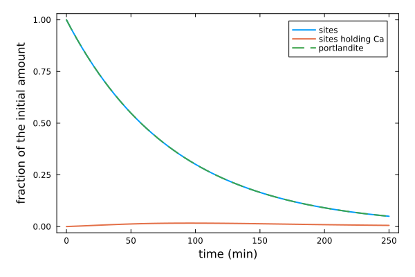
What this page does not show
That this surface is slow. The rate constant is illustrative. A rate constant fitted on an observed slow uptake is an apparent parameter, which usually stands for a transport the zero-dimensional model does not resolve (A slow surface).
A family with fast and slow states. Every state of a slow family changes through a declared reaction; a step much faster than the others is given a large constant, which makes the system stiff, rather than treated as equilibrated.