
Water and quartz from 0 to 1000 °C
Before this page
Thermochemistry, §3, for the standard state of the solvent and the domain of the HKF equations.
The standard states of the ThermoFun databases reach 1000 °C and 5000 bar: the solvent by the equation of state of water of Haar et al. (1984), the aqueous species by the HKF equations (Helgeson et al., 1981; Shock et al., 1992), the minerals by their heat-capacity functions. This page takes two equilibria that involve nothing but water and, for the second, one mineral, and compares them over that range with formulations fitted to the measurements: the ionization constant of water of Bandura and Lvov (2006) and the solubility of quartz of Manning (1994). The constants are those of slop98 (Johnson et al., 1992), the database written for this range; nothing is fitted.
1. The ionization constant of water
using ChemistryLab, DynamicQuantities, Printf
include(joinpath(pkgdir(ChemistryLab), "scripts", "water_high_temperature.jl"))

r = hw_bandura_lvov()
Δ = r.ours .- r.ref
@printf("%d states, water denser than 350 kg/m³ and at most 500 MPa\n", length(Δ))
println("  T (°C)  states   largest |Δ|   mean Δ")
for T_C in sort(unique(r.T_C))
    i = findall(==(T_C), r.T_C)
    @printf("%7.0f %7d %13.2f %+9.2f\n", T_C, length(i), maximum(abs, Δ[i]), sum(Δ[i]) / length(i))
end
175 states, water denser than 350 kg/m³ and at most 500 MPa
T (°C) states largest |Δ| mean Δ
0 12 0.30 -0.13
25 12 0.18 -0.07
50 12 0.10 -0.03
75 12 0.05 -0.01
100 11 0.02 +0.01
150 11 0.06 +0.04
200 11 0.10 +0.06
250 11 0.12 +0.07
300 11 0.16 +0.09
350 11 0.18 +0.11
400 10 0.20 +0.11
450 10 0.52 +0.10
500 9 0.27 +0.20
600 8 0.42 +0.38
700 7 0.65 +0.59
800 6 0.91 +0.83
900 6 1.20 +1.10
1000 5 1.48 +1.36using Plots
default(framestyle = :box, grid = false)
fig = plot(; xlabel = "T (°C)", ylabel = "pKw", legend = :topright, size = (700, 430))
for (k, P_MPa) in enumerate((25.0, 100.0, 300.0, 500.0))
i = findall(P -> P ≈ P_MPa * 1e6, r.P)
keep = [T for T in range(0, 1000; length = 101) if hw_density(T + 273.15, P_MPa * 1e6) >= 0.35]
plot!(fig, keep, [hw_pkw(T + 273.15, P_MPa * 1e6) for T in keep]; color = k, label = "$(Int(P_MPa)) MPa")
scatter!(fig, r.T_C[i], r.ref[i]; color = k, markersize = 3, label = false)
end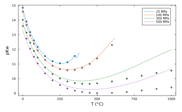
The lines are this package, the markers the formulation of Bandura and Lvov (2006). Along each isobar pKw falls with the temperature, then rises again as the expanding solvent screens the ions less.
2. The solubility of quartz
println("  T (°C)   P (bar)   log m (here)   log m (Manning)")
for (T_C, P_bar) in ((25, 1), (100, 1), (200, 500), (300, 1000), (400, 2000), (500, 2000), (600, 5000), (800, 5000))
    T, P = T_C + 273.15, P_bar * 1e5
    @printf("%7d %9d %13.3f %15.3f\n", T_C, P_bar, hw_quartz_log_m(T, P), hw_manning(T, P))
end
T (°C) P (bar) log m (here) log m (Manning)
25 1 -3.999 -4.003
100 1 -3.078 -3.059
200 500 -2.373 -2.366
300 1000 -1.878 -1.862
400 2000 -1.423 -1.402
500 2000 -1.160 -1.102
600 5000 -0.604 -0.578
800 5000 -0.234 -0.115fig2 = plot(; xlabel = "T (°C)", ylabel = "log m SiO₂(aq)", legend = :bottomright, size = (700, 430))
for (k, P_bar) in enumerate((500, 1000, 2000, 5000))
P = P_bar * 1e5
Ts = [T for T in range(25, 900; length = 90) if hw_density(T + 273.15, P) >= 0.35]
plot!(fig2, Ts, [hw_quartz_log_m(T + 273.15, P) for T in Ts]; color = k, label = "$(P_bar) bar")
plot!(fig2, Ts, [hw_manning(T + 273.15, P) for T in Ts]; color = k, linestyle = :dash, label = false)
end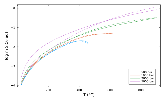
Solid lines, the database; dashed lines, the equation of Manning (1994). The two differ by 0.004 to 0.022 in