
Friedel's and Kuzel's salts from 0 to 99 °C
Before this page
CEM I 52.5 N HTS and CEM II/A-L 42.5 R from 0 to 60 °C, the same comparison on two cements without chloride.
Balonis (2019) calculated four model mixtures of tricalcium aluminate, portlandite and water with sulfate, chloride and, in two of them, calcite, from 0 to 99 °C, and stated where each chloride AFm phase gives way to monosulfate. Her Friedel's and Kuzel's salts are the records of Cemdata18 (Lothenbach et al., 2019) (her Table 1); she mixes Friedel's salt ideally with the hydroxy-AFm and with monocarbonate, which Cemdata18 does not. This page computes the same mixtures with Cemdata18 as the package ships it, Friedel's salt pure, and compares.
1. The mixtures
Each holds 0.01 mol of C₃A, 0.015 mol of portlandite and 60 ml of water, the sulfate as calcium sulfate at SO₃/Al₂O₃ = 1, the chloride as CaCl₂ at the ratio Balonis (2019) writes 2Cl/Al₂O₃ (1 for Friedel's salt), and the carbonate as calcite (data/literature/Balonis2019.json). ASSUMED: the 60 ml of water are 60 g; the activity model is the package's extended Debye–Hückel equation for a KOH solution, where the article uses Truesdell and Jones' with individual ion sizes.
using ChemistryLab, DynamicQuantities, OptimaSolver, Printf, Plots
include(joinpath(pkgdir(ChemistryLab), "scripts", "balonis2019_temperature.jl"))

cs = b19_system()
mixtures = literature_table(B19, "temperature_scans")
for (fig, cl, co2) in zip(mixtures.figure, mixtures.cl2_al2o3, mixtures.co2_al2o3)
    @printf("%-8s 2Cl/Al2O3 = %.1f, CO2/Al2O3 = %.2f\n", fig, ustrip(cl), ustrip(co2))
end
Fig. 5 2Cl/Al2O3 = 0.5, CO2/Al2O3 = 0.00
Fig. 6 2Cl/Al2O3 = 1.0, CO2/Al2O3 = 0.00
Fig. 11 2Cl/Al2O3 = 0.5, CO2/Al2O3 = 0.75
Fig. 12 2Cl/Al2O3 = 1.0, CO2/Al2O3 = 0.752. The phases from 0 to 99 °C
Each mixture every five degrees from 0 to 95 °C and at 99 °C, the volume of each phase in cm³:
scans = Dict{String, Any}()
for fig in mixtures.figure
    scans[fig] = b19_scan(cs, fig)
end
shown = ("Kuzel's salt", "Friedel's salt", "ettringite", "monosulfate", "monocarbonate", "portlandite", "total")
for fig in mixtures.figure
    println(fig, ", cm³")
    println(" °C ", join((lpad(first(p, 9), 10) for p in shown)))
    for T in (0, 10, 25, 40, 55, 70, 85, 99)
        v = b19_volumes(scans[fig], T)
        @printf("%3d %s\n", T, join((@sprintf("%10.3f", v[p]) for p in shown)))
    end
end
Fig. 5, cm³
°C Kuzel's s Friedel's ettringit monosulfa monocarbo portlandi total
0 1.758 0.433 1.639 0.000 0.000 0.455 4.285
10 1.948 0.283 1.561 0.000 0.000 0.457 4.250
25 2.309 0.000 1.414 0.000 0.000 0.462 4.184
40 2.309 0.000 1.413 0.000 0.000 0.465 4.187
55 2.264 0.000 1.387 0.059 0.000 0.468 4.178
70 1.790 0.000 1.102 0.693 0.000 0.469 4.054
85 1.020 0.000 0.612 1.735 0.000 0.469 3.836
99 0.305 0.000 0.000 2.771 0.000 0.468 3.563
Fig. 6, cm³
°C Kuzel's s Friedel's ettringit monosulfa monocarbo portlandi total
0 0.000 1.815 2.357 0.000 0.000 0.463 4.635
10 0.000 1.815 2.357 0.000 0.000 0.464 4.636
25 0.000 1.815 2.356 0.000 0.000 0.465 4.637
40 0.000 1.816 2.356 0.000 0.000 0.467 4.639
55 0.000 1.816 2.354 0.000 0.000 0.469 4.639
70 0.279 1.599 2.235 0.000 0.000 0.470 4.583
85 1.414 0.713 1.755 0.000 0.000 0.470 4.352
99 2.886 0.000 0.000 0.000 0.000 0.470 3.577
Fig. 11, cm³
°C Kuzel's s Friedel's ettringit monosulfa monocarbo portlandi total
0 0.000 0.594 3.337 0.000 0.780 0.463 5.174
10 0.000 0.622 2.875 0.000 0.939 0.463 4.956
25 0.000 0.758 2.577 0.000 0.929 0.464 4.836
40 0.000 0.879 2.459 0.000 0.859 0.466 4.802
55 2.272 0.000 1.433 0.029 0.000 0.468 4.475
70 1.794 0.000 1.113 0.683 0.000 0.469 4.336
85 1.021 0.000 0.615 1.732 0.000 0.469 4.114
99 0.305 0.000 0.000 2.771 0.000 0.468 3.840
Fig. 12, cm³
°C Kuzel's s Friedel's ettringit monosulfa monocarbo portlandi total
0 0.000 1.516 3.071 0.000 0.000 0.465 5.207
10 0.000 1.660 2.727 0.000 0.000 0.464 5.066
25 0.000 1.752 2.507 0.000 0.000 0.466 4.976
40 0.000 1.790 2.417 0.000 0.000 0.467 4.941
55 0.000 1.806 2.378 0.000 0.000 0.469 4.926
70 0.258 1.611 2.252 0.000 0.000 0.470 4.867
85 1.408 0.717 1.760 0.000 0.000 0.470 4.631
99 2.886 0.000 0.000 0.000 0.000 0.470 3.854The volumes stacked, every temperature of the scan:
layers = [p for p in keys(first(scans[first(mixtures.figure)].volumes)) if p != "total" &&
          any(fig -> any(v -> get(v, p, 0.0) > 1.0e-3, scans[fig].volumes), mixtures.figure)]
panels = map(enumerate(zip(mixtures.figure, mixtures.cl2_al2o3, mixtures.co2_al2o3))) do (k, (fig, cl, co2))
    sc = scans[fig]
    areaplot(sc.temperatures, reduce(hcat, [[get(v, p, 0.0) for v in sc.volumes] for p in layers]);
             label = permutedims(layers), palette = :tab10, lw = 0.5, legend = false,
             xlabel = "temperature (°C)", ylabel = "cm³", titlefontsize = 9,
             title = @sprintf("%s: 2Cl/Al₂O₃ %.1f, CO₂/Al₂O₃ %.2f", fig, ustrip(cl), ustrip(co2)))
end
# The legend as a panel of its own, so that the four plots keep one width.
key = plot(fill(NaN, 1, length(layers)); label = permutedims(layers), palette = :tab10, lw = 8,
           framestyle = :none, legend = :left)
plot(panels..., key; layout = @layout([grid(2, 2) a{0.17w}]), size = (1000, 720),
     left_margin = 5Plots.mm, bottom_margin = 5Plots.mm)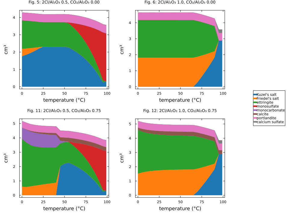
3. Where each phase gives way
The temperatures Balonis (2019) states, against the two temperatures of the scan between which the calculation loses (or forms) the phase (b19_transition):
tr = literature_table(B19, "transitions")
println("figure   phase            event   article   computed")
for (fig, phase, event, T) in zip(tr.figure, tr.phase, tr.event, tr.temperature_C)
    c = b19_transition(scans[fig], phase, event)
    computed = c === nothing ? "never" : c[2] === nothing ? "still at $(c[1]) °C" :
        c[1] === nothing ? "already at $(c[2]) °C" : "between $(c[1]) and $(c[2]) °C"
    @printf("%-8s %-16s %-6s %5.0f °C   %s\n", fig, phase, event, ustrip(T), computed)
end
figure phase event article computed
Fig. 5 Kuzel's salt last 28 °C still at 99 °C
Fig. 5 monosulfate first 28 °C between 50 and 55 °C
Fig. 5 Friedel's salt last 70 °C between 20 and 25 °C
Fig. 6 monosulfate first 60 °C never
Fig. 6 Friedel's salt last 80 °C between 90 and 95 °C
Fig. 11 monocarbonate last 50 °C between 50 and 55 °C
Fig. 11 Friedel's salt last 70 °C between 40 and 45 °C
Fig. 12 Friedel's salt last 90 °C between 90 and 95 °C
Fig. 12 ettringite last 90 °C between 90 and 95 °CThe volume lost on heating, from 0 °C to the temperatures Balonis (2019) gives it for:
sh = literature_table(B19, "shrinkage")
for (fig, p) in zip(sh.figure, sh.percent)
    v(T) = b19_volumes(scans[fig], T)["total"]
    @printf("%-8s article %2.0f %%, computed %4.1f %% at 90 °C and %4.1f %% at 99 °C\n", fig, ustrip(p),
            100 * (1 - v(90) / v(0)), 100 * (1 - v(99) / v(0)))
end
Fig. 5 article 15 %, computed 12.9 % at 90 °C and 16.9 % at 99 °C
Fig. 6 article 23 %, computed 8.0 % at 90 °C and 22.8 % at 99 °C
Fig. 11 article 30 %, computed 22.5 % at 90 °C and 25.8 % at 99 °C
Fig. 12 article 25 %, computed 12.8 % at 90 °C and 26.0 % at 99 °C4. Why Kuzel's salt stays
Kuzel's salt is half monosulfate and half Friedel's salt, and one water: C4AsClH12 = ½ monosulphate12 + ½ C4AClH10 + H2O. The Gibbs energy of that reaction, from the four records, says at which temperature the two AFm phases would take over from it, pure:
g(s, T) = ustrip(us"kJ/mol", B19_DB[s][:ΔₐG⁰](T = (T + 273.15) * u"K", P = 1.0e5u"Pa"; unit = true))
ΔrG(T) = g("monosulphate12", T) / 2 + g("C4AClH10", T) / 2 + g("H2O@", T) - g("C4AsClH12", T)
for T in (0, 25, 55, 85, 99)
    @printf("%3d °C  ΔrG = %+.2f kJ/mol\n", T, ΔrG(T))
end
0 °C ΔrG = +1.83 kJ/mol
25 °C ΔrG = +1.59 kJ/mol
55 °C ΔrG = +1.19 kJ/mol
85 °C ΔrG = +0.65 kJ/mol
99 °C ΔrG = +0.34 kJ/mol5. What the comparison says
Where chloride is plentiful, the calculation follows Balonis (2019). With 2Cl/Al₂O₃ = 1, Friedel's salt goes between 90 and 95 °C, where the article states 80 and about 90 °C, ettringite with it in the carbonate mixture, and the solids have lost 22.8 and 26.0 % of their volume at 99 °C, against the article's 23 and 25 %. The monocarbonate of the carbonate mixture with less chloride goes between 50 and 55 °C, where the article states about 50.
Where it is scarce, Kuzel's salt takes the place of the phases of Balonis (2019). With 2Cl/Al₂O₃ = 0.5 the calculation keeps Kuzel's salt up to 99 °C and loses Friedel's salt by 25 °C (by 45 °C with carbonate), where the article keeps Kuzel's salt up to 28 °C only and Friedel's salt up to 70 °C; its monosulfate appears between 50 and 55 °C instead of about 28. With 2Cl/Al₂O₃ = 1 Kuzel's salt forms above 55 °C, where the article forms monosulfate from 60 °C. Of the same records, the reaction of Section 4 costs Kuzel's salt 1.6 kJ/mol at 25 °C and 0.3 at 99 °C, never zero below 100 °C, so pure phases keep it. The article's Friedel's salt and hydroxy-AFm are solid solutions, which lower the competing AFm phases by about as much: the ideal mixing of two members at equal fractions is worth RT ln 2, 1.7 kJ/mol at 25 °C. The package does not declare those solutions; a calculation that needs the article's Kuzel's salt must declare them in its system.
Where to go next
CEM I 52.5 N HTS and CEM II/A-L 42.5 R from 0 to 60 °C finds the same transition from ettringite and monocarbonate to monosulfate in two cements, and Solid solutions writes the mixing Balonis (2019) adds.