The cements of Lavergne et al. (2018): degrees of hydration, phase volumes and heat

Before this page

A complete CEM I 52.5 N, through its pore solution, whose model this page runs on the cement of the article.

Lavergne et al. (2018) estimate the mechanical properties of hydrating cement pastes from a hydration model: the kinetic law of Parrott and Killoh (1984) for each clinker phase, a set of stoichiometric reactions for the hydrates, and an energy balance for the temperature. Before the mechanics, they check that model against measurements from the literature and from their own laboratory: degrees of hydration of the clinker phases by X-ray diffraction, heat in isothermal and semi-adiabatic calorimeters. This page takes those comparisons one by one and puts the package's calculation beside each: the same kinetic law where the article uses it, and, for what the hydrates are, a Gibbs minimization in place of the stoichiometric reactions.

Every number the page compares with is read from the article: the compositions of its Table 7, the curves of its figures read exactly from their vector drawings, measured points and model estimates alike (data/literature/Lavergne2018.json).

Questions this page answers

• How close does the package's Parrott–Killoh law come to the article's estimates, and to the measured degrees of hydration?

• What phases does a Gibbs minimization give a CEM I paste as it hydrates, against the stoichiometric reactions of the article?

• How much heat do the cements of Lerch and Ford release in their first three days, and at what temperature does the model drift from the measurement?

• What does silica fume in place of part of the cement change in the phases of the paste?

• How does the same paste heat a semi-adiabatic calorimeter, and what changes when limestone or silica fume replaces part of the cement?

The cements

The article gathers in its Table 7 the cements of every test it reproduces: their Bogue composition, their calcium sulfates and their Blaine fineness. The first seven serve the degrees of hydration below.

using ChemistryLab, DynamicQuantities, OptimaSolver, OrdinaryDiffEq, Printf, Plots, Logging
gr()

t7 = literature_table("Lavergne2018", "table7_cements")
row(c) = findfirst(==(c), t7.name)
println("cement   C3S   C2S   C3A  C4AF  sulfates        Blaine (m²/kg)")
for c in ("A", "B", "C", "OPCN", "OPCS", "OPC", "CRC")
    i = row(c)
    pct(x) = ismissing(x) ? "    –" : @sprintf("%5.1f", x)
    @printf("%-6s %s %s %s %s  %-14s  %.1f\n", c, pct(t7.C3S[i]), pct(t7.C2S[i]),
            pct(t7.C3A[i]), pct(t7.C4AF[i]), t7.calcium_sulfates[i], ustrip(us"m^2/kg", t7.blaine[i]))
end

cement   C3S   C2S   C3A  C4AF  sulfates        Blaine (m²/kg)
A       68.0  25.3   3.6     –  3.9             470.0
B       49.1  25.5   5.8  10.7  4.3             310.0
C       64.5  16.2   6.7   8.7  3.3             200.0
OPCN    71.6  10.9   3.7  10.7  3.1             376.5
OPCS    65.6  16.4   8.0   7.4  2.6             359.8
OPC     52.5  18.2   5.0  10.9  0.4+ 2.2CS̅      380.0
CRC     67.6  13.1   2.7   8.9  2.4CS̅H0.5+ 1.2CS̅  350.0

Degrees of hydration of the clinker phases

Each clinker phase hydrates by the law of Parrott and Killoh (1984), the slowest of three rates: nucleation and growth, diffusion through the hydrates, and the formation of a shell around the grain, with the parameters of the article's Table 3 (PK84_PARAMS_C3S and its siblings). The rate scales with the Blaine fineness of the cement and, through the activation energy of each phase (Table 4), with the temperature (parrott_killoh_avrami). The degree of a phase at any time follows by integrating that rate alone, as the article does: no other phase and no hydrate enters it.

const PK = Dict("C3S" => PK84_PARAMS_C3S, "C2S" => PK84_PARAMS_C2S,
                "C3A" => PK84_PARAMS_C3A, "C4AF" => PK84_PARAMS_C4AF)

# The degree of hydration of one clinker phase of a cement of Blaine fineness B,
# at the times `days`, under the temperature history T(t) (t in seconds, T in K).
function pk_degree(phase, B, T, days)
    law = parrott_killoh_avrami(PK[phase], phase; blaine = B)
    idx = Dict(phase => 1)
    n0, lna = StateView([1.0], idx), StateView([0.0], idx)
    f(n, _, t) = [-law(T(t), 1.0e5, t, StateView(n, idx), lna, n0)]
    sol = solve(ODEProblem(f, [1.0], (0.0, 86400 * maximum(days))), Rodas5P();
                abstol = 1.0e-12, reltol = 1.0e-9)
    return [1 - sol(86400 * d)[1] for d in days]
end

Lavergne et al. (2018), Fig. 4 compares that law with the degrees measured by XRD/Rietveld analysis on three cements, A, B and C, at 20 °C. Below, the package's integration (solid lines), the article's own estimate (dashed) and the measurements (markers), on the four clinker phases:

PHASES = ("C3S", "C3A", "C2S", "C4AF")
days = 10 .^ range(-1, 3; length = 120)
at20(t) = 293.15

function degree_panels(meas, est, groups; T = g -> at20, label = g -> g.name, title = "")
    panels = map(PHASES) do ph
        p = plot(; xscale = :log10, xlims = (0.1, 1000), ylims = (0, 1), legend = false,
                 title = ph, xlabel = "t [days]", ylabel = "α")
        for (k, g) in enumerate(groups)
            c = palette(:tab10)[k]
            sm(t) = [i for i in eachindex(t.phase) if t.phase[i] == ph && g.select(t, i)]
            ie, im = sm(est), sm(meas)
            isempty(ie) && isempty(im) && continue
            plot!(p, days, pk_degree(ph, g.blaine, T(g), days); color = c, lw = 2, label = label(g))
            plot!(p, ustrip.(u"d", est.time[ie]), est.alpha[ie]; color = c, ls = :dash, label = "")
            scatter!(p, ustrip.(u"d", meas.time[im]), meas.alpha[im]; color = c, ms = 3, label = "")
        end
        p
    end
    plot(panels...; layout = (2, 2), size = (860, 640), legend = :topleft,
         plot_title = title, left_margin = 4Plots.mm, bottom_margin = 4Plots.mm)
end

fig4m = literature_table("Lavergne2018", "fig4_hydration_degree_measured")
fig4e = literature_table("Lavergne2018", "fig4_hydration_degree_estimated")
cements4 = [(name = c, blaine = t7.blaine[row(c)], select = (t, i) -> t.cement[i] == c) for c in ("A", "B", "C")]
degree_panels(fig4m, fig4e, cements4; label = g -> "cement " * g.name,
              title = "Fig. 4: computed (solid), the article's estimate (dashed), measured")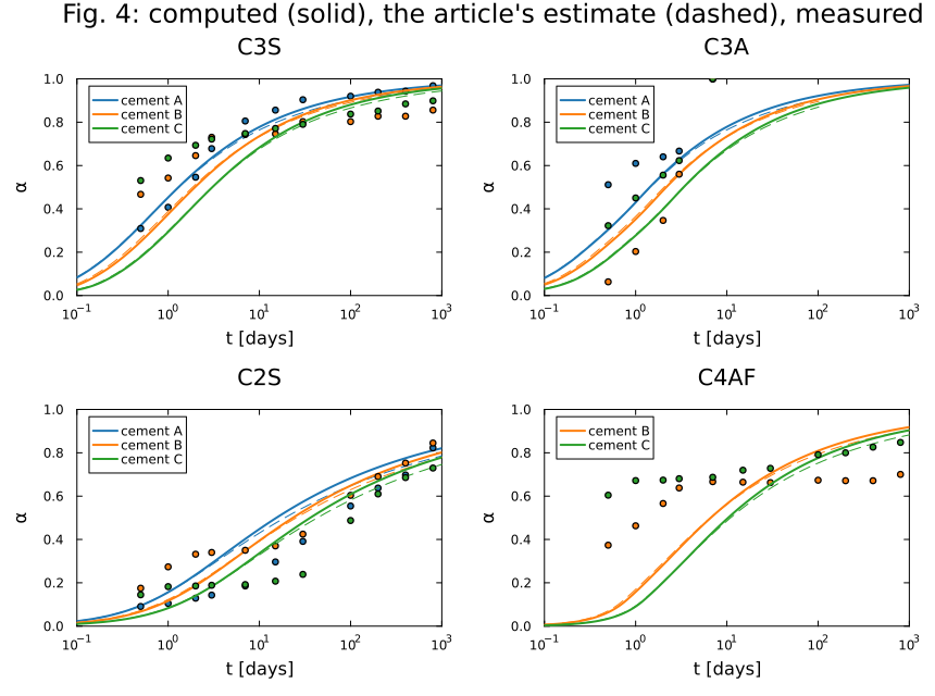

The two integrations of the same law agree to a few hundredths. The measurements are another matter, as the article says itself: the law has the right characteristic times for C₃S, C₂S and C₃A, but its degree can be off by 0.2 or more, and its C₄AF is uncertain on both sides, model and measurement.

# The largest difference with the article's estimate, phase by phase.
function gap(meas, est, groups; T = g -> at20)
    out = Dict{String, Float64}()
    for g in groups, ph in PHASES
        ie = [i for i in eachindex(est.phase) if est.phase[i] == ph && g.select(est, i)]
        isempty(ie) && continue
        d = maximum(abs.(pk_degree(ph, g.blaine, T(g), ustrip.(u"d", est.time[ie])) .- est.alpha[ie]))
        out[ph] = max(get(out, ph, 0.0), d)
    end
    return out
end
for (ph, d) in sort(collect(gap(fig4m, fig4e, cements4)); by = first)
    @printf("%-5s largest |Δα| with the article's estimate: %.3f\n", ph, d)
end

C2S   largest |Δα| with the article's estimate: 0.037
C3A   largest |Δα| with the article's estimate: 0.017
C3S   largest |Δα| with the article's estimate: 0.017
C4AF  largest |Δα| with the article's estimate: 0.024

Away from 20 °C

Lavergne et al. (2018), Fig. 5 take the measurements of two cements, OPCN and OPCS, cured at 20 °C for a day and then stored at 10, 20, 30 or 40 °C. The same law follows the temperature through the activation energy of each phase:

fig5m = literature_table("Lavergne2018", "fig5_hydration_degree_measured")
fig5e = literature_table("Lavergne2018", "fig5_hydration_degree_estimated")
history(Tc) = t -> t < 86400 ? 293.15 : Tc + 273.15
cured(c) = [(name = "$(Int(Tc)) °C", Tc = Tc, blaine = t7.blaine[row(c)],
             select = (t, i) -> t.cement[i] == c && t.temperature_C[i] == Tc) for Tc in (10.0, 20.0, 30.0, 40.0)]
degree_panels(fig5m, fig5e, cured("OPCN"); T = g -> history(g.Tc), label = g -> g.name,
              title = "Fig. 5, OPCN: computed (solid), the article's estimate (dashed), measured")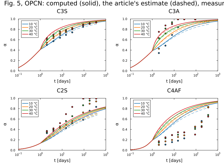

degree_panels(fig5m, fig5e, cured("OPCS"); T = g -> history(g.Tc), label = g -> g.name,
              title = "Fig. 5, OPCS: computed (solid), the article's estimate (dashed), measured")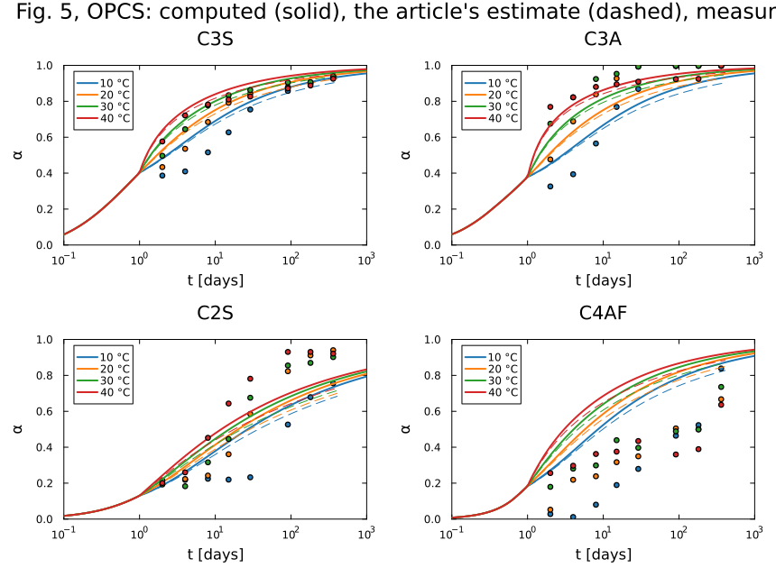

The temperature moves the computed degrees as it moves the measured ones, which is what the activation energies of Table 4 are for; the article's estimate and this integration stay within a few hundredths of each other again.

Two more cements

Lavergne et al. (2018), Fig. 6 end with an ordinary cement and a cement of another composition, OPC and CRC:

fig6m = literature_table("Lavergne2018", "fig6_hydration_degree_measured")
fig6e = literature_table("Lavergne2018", "fig6_hydration_degree_estimated")
cements6 = [(name = c, blaine = t7.blaine[row(c)], select = (t, i) -> t.cement[i] == c) for c in ("OPC", "CRC")]
degree_panels(fig6m, fig6e, cements6; title = "Fig. 6: computed (solid), the article's estimate (dashed), measured")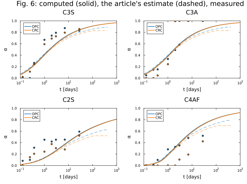

for (ph, d) in sort(collect(gap(fig6m, fig6e, cements6)); by = first)
    @printf("%-5s largest |Δα| with the article's estimate: %.3f\n", ph, d)
end

C2S   largest |Δα| with the article's estimate: 0.240
C3A   largest |Δα| with the article's estimate: 0.122
C3S   largest |Δα| with the article's estimate: 0.121
C4AF  largest |Δα| with the article's estimate: 0.196

Here the two calculations part by up to a quarter, and the figure shows where: the article's estimates level off and stop rising after about a hundred days, which is what its model does when the internal relative humidity of the paste falls below 80 % (its Eq. 10). That term, which depends on the water to cement ratio of a test the article does not give, is left out of the integration above; before the article's curves level off, the two agree to a few hundredths.

The phases of a hydrating paste

The kinetic law says how much of each clinker phase has reacted, not what it has become. The article answers with stoichiometric reactions written in advance (its Table 2); the package answers with a Gibbs minimization of everything that is not clinker, at every step of the integration (A complete CEM I 52.5 N, through its pore solution). The paste of Lavergne et al. (2018), Fig. 1, left, is that of their own cement, the CEM I 52.5 N of Table 9, at w/c = 0.5 and sealed; the package's model of that cement runs here for a year.

include(joinpath(pkgdir(ChemistryLab), "scripts", "ionic_hydration.jl"))
quiet(f) = with_logger(f, NullLogger())
paste = quiet() do
    run_ionic_hydration(; wb = 0.5, tend = 365 * 86400.0)
end
tdays = [0.1, 0.25, 0.5, 0.75, 1, 1.5, 2, 3, 5, 7, 10, 14, 28, 56, 90, 180, 365]
states = quiet() do
    speciated_states(paste.sol, paste.kp; times = tdays .* 86400)
end
_, fractions, _, _ = ionic_phase_history(paste, tdays .* 86400; states)

# The degree of hydration of the cement: the mass of clinker consumed.
clinker = ("C3S", "C2S", "C3A", "C4AF")
M = Dict(c => ustrip(us"kg/mol", paste.cs[c][:M]) for c in clinker)
clinker_mass(st) = sum(ustrip(us"mol", moles(st, c)) * M[c] for c in clinker)
α = [1 - clinker_mass(st) / clinker_mass(paste.state0) for st in states]
@printf("%s; α = %.2f after 28 days, %.2f after a year\n", paste.sol.retcode, α[13], α[end])

Success; α = 0.80 after 28 days, 0.92 after a year

The article's phases and the package's families are put side by side: its "Aft, Afm" are the ettringite and the AFm phases, its C-S-H gel holds its gel water, as the package's does, and its "air" is the empty porosity a sealed paste gains as it shrinks. The package's hydrogarnet and iron hydroxide, which the article does not draw, are left out of the comparison.

fig1 = literature_table("Lavergne2018", "fig1_volume_fractions_estimated")
families = [
    "unhydrated cement" => ["anhydrous"], "gypsum" => ["gypsum"], "calcite" => ["calcite"],
    "Aft, Afm" => ["AFt", "AFm"], "Portlandite" => ["CH"], "C-S-H gel" => ["C-S-H"],
    "capillary water" => ["water"],
]
push!(families, "air" => ["void"])
mine(f, keys) = sum(get(f, k, 0.0) for k in keys)
theirs(name; paste = "plain paste, w/c = 0.5") =
    (i = [j for j in eachindex(fig1.phase) if fig1.paste[j] == paste && fig1.phase[j] == name];
     (fig1.alpha[i], fig1.volume_fraction[i]))
panels = map(families) do (name, keys)
    a, v = theirs(name)
    p = plot(a, v; color = :black, ls = :dash, label = "article",
             title = name, xlabel = "α", ylabel = "volume fraction", xlims = (0, 1), legend = false)
    plot!(p, α, [mine(f, keys) for f in fractions]; color = :steelblue, lw = 2, marker = :circle, ms = 3, label = "computed")
end
plot(panels...; layout = (2, 4), size = (1000, 520), plot_title = "Fig. 1, left: computed (blue), the article's model (dashed)",
     left_margin = 3Plots.mm, bottom_margin = 4Plots.mm)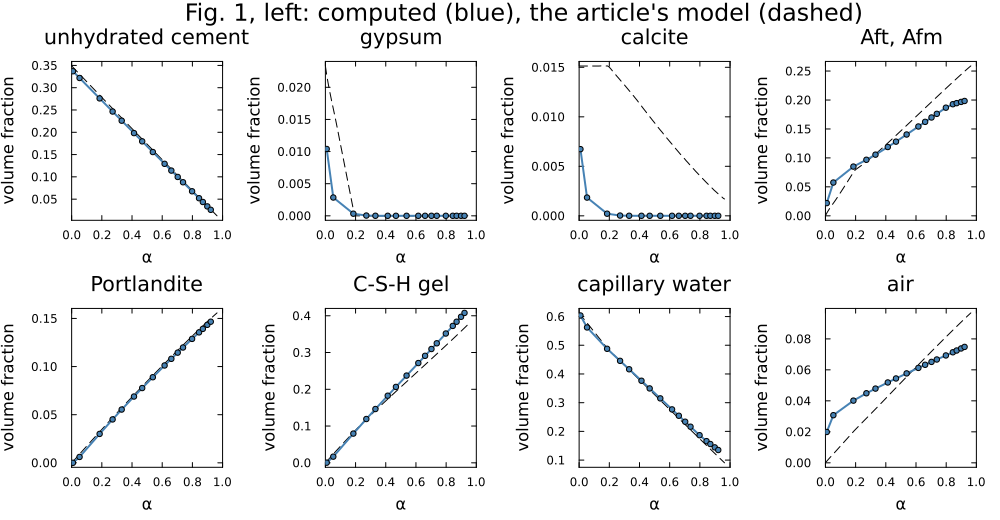

At the degree the paste reaches in 28 days, the two compositions read, in fractions of the volume of the fresh paste (the article's curve taken between its two nearest vertices):

k28 = findfirst(==(28), tdays)
interp(x, xs, ys) = (j = searchsortedlast(xs, x); j == length(xs) ? ys[end] :
                     ys[j] + (ys[j + 1] - ys[j]) * (x - xs[j]) / (xs[j + 1] - xs[j]))
@printf("α = %.2f\n%-18s %9s %9s\n", α[k28], "", "computed", "article")
for (name, keys) in families
    a, v = theirs(name)
    @printf("%-18s %9.3f %9.3f\n", name, mine(fractions[k28], keys), interp(α[k28], a, v))
end

α = 0.80
                    computed   article
unhydrated cement      0.068     0.070
gypsum                 0.000     0.000
calcite                0.000     0.004
Aft, Afm               0.187     0.220
Portlandite            0.129     0.132
C-S-H gel              0.352     0.319
capillary water        0.187     0.175
air                    0.069     0.081

The anhydrous cement, the portlandite and the capillary water agree within a hundredth of the volume. The minimization puts more of it in the C-S-H gel and less in the AFt and AFm phases and in the empty porosity. The early sulfate and carbonate phases tell the two approaches apart most: the minimization consumes the calcite at once, into carboaluminates, and the gypsum from the first hours, where the reactions of the article form ettringite while gypsum lasts and then monocarboaluminate while calcite does, so that its calcite lasts to the end.

With silica fume

Lavergne et al. (2018), Fig. 1, right, draws the same cement with a tenth of its mass replaced by silica fume, at w/(c+sf) = 0.35. The model of the paste takes the fume of Table 7 (lavergne_addition in the script): its silica as amorphous silica, Amor-Sl, dissolving by the law of Waller (1999) with the parameters of the article, Eqs. (24) and (25) at a Blaine fineness of 2000 m²/kg, up to its pozzolanic activity, 0.9 of it; the rest of the fume, 5.5 %, is left out. Beside the jennite end member of the C-S-H the minimization may form the tobermorite one, Tob-II, of Ca/Si 0.83, where the pozzolanic reaction of the article forms C₁.₁SH₃.₉ (its Table 1), and the gel water of each is counted with it as the formulas of the article give it. The article's curves stop at α = 0.66, which the paste reaches within a month.

sf = lavergne_addition("SF", 0.1)
sfpaste = quiet() do
    run_ionic_hydration(; wb = 0.35, gypsum = 0.9 * IONIC_CEMENT.gypsum, filler = 0.9 * IONIC_CEMENT.filler,
                        silica_fume = sf, tend = 28 * 86400.0)
end
tsf = tdays[tdays .<= 28]
sfstates = quiet() do
    speciated_states(sfpaste.sol, sfpaste.kp; times = tsf .* 86400)
end
_, sffractions, _, _ = ionic_phase_history(sfpaste, tsf .* 86400; states = sfstates)
αsf = [1 - clinker_mass(st) / clinker_mass(sfpaste.state0) for st in sfstates]
silica(st) = ustrip(us"mol", moles(st, "Amor-Sl"))
@printf("%s; after 28 days α = %.2f, %.2f of the silica reacted, portlandite %.2f mol, tobermorite %.2f mol\n",
        sfpaste.sol.retcode, αsf[end], 1 - silica(sfstates[end]) / silica(sfpaste.state0),
        ustrip(us"mol", moles(sfstates[end], "Portlandite")), ustrip(us"mol", moles(sfstates[end], "Tob-II")))

Success; after 28 days α = 0.68, 0.55 of the silica reacted, portlandite 0.95 mol, tobermorite 0.00 mol

sfpaste_name = "10 % silica fume, w/(c+sf) = 0.35"
sffamilies = [families[1], "silica fume" => ["silica fume"], families[2:end]...]
panels = map(sffamilies) do (name, keys)
    a, v = theirs(name; paste = sfpaste_name)
    p = plot(a, v; color = :black, ls = :dash, label = "article",
             title = name, xlabel = "α", ylabel = "volume fraction", xlims = (0, 0.8), legend = false)
    plot!(p, αsf, [mine(f, keys) for f in sffractions]; color = :steelblue, lw = 2, marker = :circle, ms = 3, label = "computed")
end
plot(panels...; layout = (3, 3), size = (1000, 760), plot_title = "Fig. 1, right: computed (blue), the article's model (dashed)",
     left_margin = 3Plots.mm, bottom_margin = 4Plots.mm)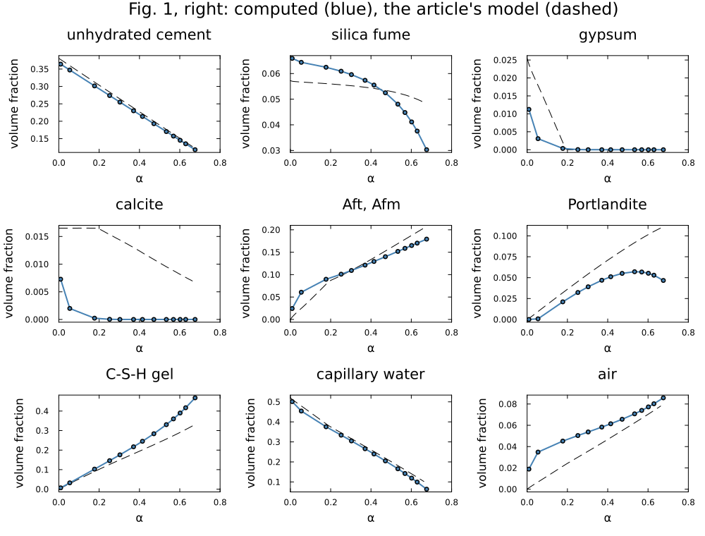

At the last degree the paste reaches below the end of the article's curves:

k = findlast(<=(0.66), αsf)
@printf("α = %.2f, after %g days\n%-18s %9s %9s\n", αsf[k], tsf[k], "", "computed", "article")
for (name, keys) in sffamilies
    a, v = theirs(name; paste = sfpaste_name)
    @printf("%-18s %9.3f %9.3f\n", name, mine(sffractions[k], keys), interp(αsf[k], a, v))
end

α = 0.63, after 14 days
                    computed   article
unhydrated cement      0.135     0.140
silica fume            0.038     0.050
gypsum                 0.000     0.000
calcite                0.000     0.008
Aft, Afm               0.170     0.195
Portlandite            0.053     0.105
C-S-H gel              0.417     0.305
capillary water        0.099     0.123
air                    0.080     0.074

After 28 days the cement has reached α = 0.68 and 55 % of the silica of the fume has reacted, and the portlandite has not run out. In equilibrium with portlandite the C-S-H of the minimization is the jennite end member, of Ca/Si 1.67, and the tobermorite one never forms: the pozzolanic reaction of the calculation takes 1.67 mol of portlandite per mole of silica, where that of the article, 1.1 CH + S + 2.8 H → C₁.₁SH₃.₉, takes 1.1. The computed portlandite therefore peaks near α = 0.55 and falls, half the article's at α = 0.63, and the C-S-H gel is a third larger. The fume reacts faster in the calculation than in the article's model as well, by the law and the parameters the article gives, its volume 0.038 against 0.050 at that degree.

The heat of hydration in isothermal calorimeters

The heat a paste releases at constant temperature is the other measurement the article checks its model against. Lerch and Ford (1948) measured it on pastes of the 27 cements of a long-time study, at w/c = 0.4, in calorimeters held at four temperatures, from one hour to three days; Lavergne et al. (2018), Fig. 7 put their model beside those measurements, one panel per ASTM type of cement. The model of the paste above runs here on the compositions of Table 7, in an isothermal calorimeter, and the heat is the enthalpy the paste has lost since mixing (cumulative_heat).

Two choices make the comparison possible. The cements of Lerch and Ford carry their sulfate as anhydrite, and the model of the paste knows gypsum only: each cement enters with the gypsum that carries the same sulfate, the ratio of the two taken from the molar masses of the phases. And one kilogram of cement is run, so that the heat comes in joules per gram of cement, as the article plots it.

# Kilograms of gypsum that carry the sulfate of one kilogram of anhydrite.
molar_mass(formula) = ustrip(us"kg/mol", Species(formula)[:M])
gypsum_per_anhydrite = (molar_mass("CaSO4") + 2 * molar_mass("H2O")) / molar_mass("CaSO4")

# The heat a paste of one kilogram of the cement `c` of Table 7 releases over
# `days` at the water-to-cement ratio `wc`, in an isothermal calorimeter at
# `Tc` °C: the times in days and the heat in J/g of cement.
function isothermal_heat(c, Tc; wc = 0.4, days = 3)
    i = row(c)
    s = parse(Float64, replace(t7.calcium_sulfates[i], "CS̅" => "")) / 100
    g = s * gypsum_per_anhydrite       # kg of gypsum for the anhydrite of 1 kg of cement
    binder = 1 - s + g                 # kg of clinker and gypsum
    f = 100 * (1 - s)                  # Table 7 gives percent of cement, the model fractions of clinker
    clinker = (C3S = t7.C3S[i] / f, C2S = t7.C2S[i] / f, C3A = t7.C3A[i] / f, C4AF = t7.C4AF[i] / f)
    cal = IsothermalCalorimeter((Tc + T_ZERO_CELSIUS)u"K")
    run = quiet() do
        run_ionic_hydration(; wb = wc / binder, binder_mass = binder * u"kg", clinker,
                            gypsum = g / binder, filler = 0.0, blaine = t7.blaine[i],
                            calorimeter = cal, tend = days * 86400.0)
    end
    t, Q = cumulative_heat(run.sol, cal)
    return (; days = t ./ 86400, heat = Q ./ 1000)
end

# The rows of Fig. 7 for one cement at one temperature: times in days, heat in J/g.
fig7m = literature_table("Lavergne2018", "fig7_heat_measured")
fig7e = literature_table("Lavergne2018", "fig7_heat_estimated")
function fig7(tab, c, Tc)
    k = [i for i in eachindex(tab.cement) if tab.cement[i] == c && abs(tab.temperature_C[i] - Tc) < 1]
    return ustrip.(u"d", tab.time[k]), ustrip.(u"J/g", tab.heat[k])
end

Panels (a) to (d) of the figure give each type at 4, 23, 32 and 40 °C; panel (e) gives the same four temperatures to a tenth of a degree, 4.4, 23.9, 32.2 and 40.6 °C, which the calculation takes. The first cement of each type, at 23.9 °C, computed (solid lines), as the article estimates it (dashed) and measured (markers):

types = ["c11" => "I", "c21" => "II", "c31" => "III", "c41" => "IV", "c51" => "V"]
at23 = Dict(c => isothermal_heat(c, 23.9) for (c, _) in types)
println("cement  type      Q at 1 day (J/g)             Q at 3 days (J/g)")
println("                measured computed article   measured computed article")
for (c, ty) in types
    tm, Qm = fig7(fig7m, c, 23.9)
    te, Qe = fig7(fig7e, c, 23.9)
    r = at23[c]
    at(t) = (Qm[argmin(abs.(tm .- t))], interp(t, r.days, r.heat), interp(t, te, Qe))
    @printf("%-6s  %-4s    %7.1f  %7.1f  %7.1f    %7.1f  %7.1f  %7.1f\n", c, ty, at(1)..., at(3)...)
end

cement  type      Q at 1 day (J/g)             Q at 3 days (J/g)
                measured computed article   measured computed article
c11     I         182.4    176.6    185.5      296.6    265.9    258.8
c21     II        132.6    127.9    132.4      212.5    204.9    196.4
c31     III       242.7    228.5    233.9      350.2    309.5    297.2
c41     IV        138.5    107.0    107.0      210.9    163.6    154.9
c51     V         157.3    133.1    138.8      212.5    204.1    196.9

p = plot(; xlabel = "t [days]", ylabel = "Q [J/g of cement]", xlims = (0, 3), ylims = (0, 400),
         legend = :topleft, size = (720, 420),
         title = "first cement of each type, 23.9 °C")
for (k, (c, ty)) in enumerate(types)
    col = palette(:tab10)[k]
    tm, Qm = fig7(fig7m, c, 23.9)
    te, Qe = fig7(fig7e, c, 23.9)
    plot!(p, at23[c].days, at23[c].heat; color = col, lw = 2, label = "$c, type $ty")
    plot!(p, te, Qe; color = col, ls = :dash, label = "")
    scatter!(p, tm, Qm; color = col, ms = 3, label = "")
end
p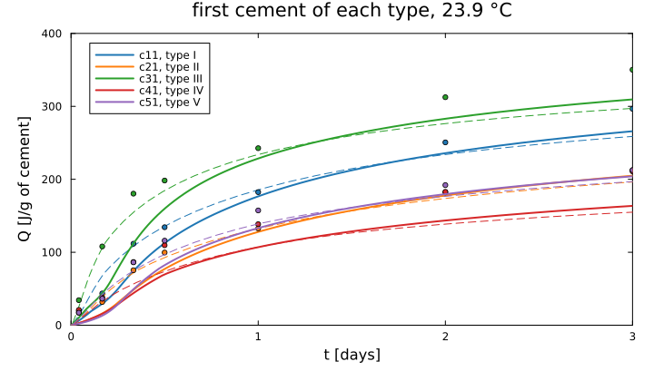

The two calculations share the kinetic law of the clinker phases and differ in what the phases become, a Gibbs minimization against stoichiometric reactions, and in the start: the model of the paste holds the silicates in a dormant period, five hours long and the same at every temperature (A complete CEM I 52.5 N, through its pore solution), where the law alone starts at once. Panel (e) follows cement c51, of type V, through the four temperatures, drawn as above:

temps = [4.4, 23.9, 32.2, 40.6]
c51 = Dict(Tc => (Tc == 23.9 ? at23["c51"] : isothermal_heat("c51", Tc)) for Tc in temps)
rms(x) = sqrt(sum(abs2, x) / length(x))
p = plot(; xlabel = "t [days]", ylabel = "Q [J/g of cement]", xlims = (0, 3), ylims = (0, 400),
         legend = :topleft, size = (720, 420),
         title = "cement c51, type V")
for (k, Tc) in enumerate(temps)
    col = palette(:tab10)[k]
    tm, Qm = fig7(fig7m, "c51", Tc)
    te, Qe = fig7(fig7e, "c51", Tc)
    plot!(p, c51[Tc].days, c51[Tc].heat; color = col, lw = 2, label = "$Tc °C")
    plot!(p, te, Qe; color = col, ls = :dash, label = "")
    scatter!(p, tm, Qm; color = col, ms = 3, label = "")
    @printf("%4.1f °C: root-mean-square gap to the seven measurements, computed %4.1f J/g, article %4.1f J/g\n",
            Tc, rms([interp(t, c51[Tc].days, c51[Tc].heat) for t in tm] .- Qm),
            rms([interp(t, te, Qe) for t in tm] .- Qm))
end
p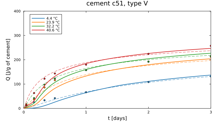

Within the first day the paste model releases its heat later than the calorimeter and than the article's estimate: its dormant period holds the silicates through the first hours, when the measurement already sees them react. From one day on the two calculations run side by side, the package's 7 to 12 J/g above the article's at three days, the enthalpy of what the minimization forms rather than that of the reactions, and both fall short of the heat measured on the cements of types I, III and IV, by 31, 41 and 47 J/g for the package. Cement c41 is the plainest case: at one day the two calculations agree to the tenth, 107.0 J/g, and both miss 31 J/g of the measurement, a gap in the kinetic law they share rather than in what either makes of it. Through the four temperatures, the package stays 15 to 24 J/g from the measured heat of cement c51 in root mean square, against 9 to 14 J/g for the article's estimate, the largest gap at 23.9 °C around half a day.

Lavergne et al. (2018), Fig. 9(b) adds a warmer calorimeter: the heat of a mortar of cement ca of Table 7, at w/c = 0.55, held at 20, 30 and 50 °C, from the work of Waller (1999). The same calculation, over five days:

fig9m = literature_table("Lavergne2018", "fig9b_heat_measured")
fig9e = literature_table("Lavergne2018", "fig9b_heat_estimated")
temps9 = [20.0, 30.0, 50.0]
ca55 = Dict(Tc => isothermal_heat("ca", Tc; wc = 0.55, days = 5) for Tc in temps9)
p = plot(; xlabel = "t [days]", ylabel = "Q [J/g of cement]", xlims = (0, 5), ylims = (0, 450),
         legend = :bottomright, size = (720, 420), title = "mortar ca55")
for (k, Tc) in enumerate(temps9)
    col = palette(:tab10)[k]
    sel(tab) = [i for i in eachindex(tab.time) if tab.temperature_C[i] == Tc]
    km, ke = sel(fig9m), sel(fig9e)
    tm, Qm = ustrip.(u"d", fig9m.time[km]), ustrip.(u"J/g", fig9m.heat[km])
    te, Qe = ustrip.(u"d", fig9e.time[ke]), ustrip.(u"J/g", fig9e.heat[ke])
    plot!(p, ca55[Tc].days, ca55[Tc].heat; color = col, lw = 2, label = "$Tc °C")
    plot!(p, te, Qe; color = col, ls = :dash, label = "")
    scatter!(p, tm, Qm; color = col, ms = 3, label = "")
    @printf("%4.1f °C, at %.1f days: measured %5.1f J/g, computed %5.1f, article %5.1f\n", Tc, tm[end], Qm[end],
            interp(tm[end], ca55[Tc].days, ca55[Tc].heat), interp(tm[end], te, Qe))
end
p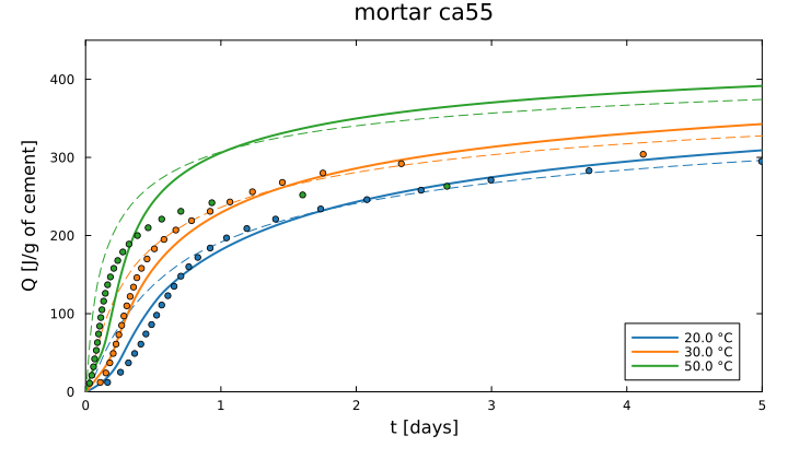

At 20 °C the calculation ends 14 J/g above the measurement at five days, where the article's estimate meets it. The warmer the calorimeter, the further both overshoot: by 28 and 15 J/g at 30 °C, and by 102 and 89 J/g at 50 °C, where the measured heat stays near 250 to 260 J/g from a day and a half on while both calculations climb past 350 J/g. An overshoot the two share, and which grows with the temperature, points to the kinetic law and its activation energies, common to both, rather than to what either makes of the reactions. In the first hours, as above, the dormant period of the model of the paste delays its heat at every temperature.

Mortars of CEM I 52.5 N in a semi-adiabatic calorimeter, inside the kinetics

The calorimeters of Lerch and Ford hold the paste at one temperature, and what they record is read off the calculated trajectory as the enthalpy the paste loses. A semi-adiabatic calorimeter cannot be read that way. It lets the heat of hydration raise the temperature of the sample against the losses of the vessel, and the temperature raises the rates of the reactions in turn. The temperature is then an unknown of the kinetic problem: the enthalpy of the cell, the paste over its whole composition and the vessel, changes only by what leaves through the walls, and the temperature is the root of that balance, solved with the equilibrium of the paste at every evaluation (The semi-adiabatic cell). The losses of the vessel are quadratic in the temperature difference,     .

This section reproduces the test of Lavergne et al. (2018) on the plain-cement mortar C100 at w/b = 0.5, in their calorimeter, with the model of the paste above and nothing adjusted.

The cell

The cell is NF EN 196-9's, as Lavergne et al. (2018) calibrated it: their Eq. (23) for the losses, their Table 11 for the mix. The sand keeps the temperature moderate and takes no part in the chemistry; it enters with the vessel and the water it absorbs as a fixed heat capacity, while the paste's own heat capacity is summed over its composition at every step.

mix = CALORIMETRY_MIX_C100
T_env = 293.15u"K"
cell = semiadiabatic_cell(; mix, T0 = T_env, T_env)
@printf("mortar: %.0f g binder, %.0f g sand, %.0f g water, of which %.1f g in the sand (w/b %.3f)\n",
        ustrip(us"g", mix.binder), ustrip(us"g", mix.sand), ustrip(us"g", mix.water),
        ustrip(us"g", mix.absorbed), mix.wb)
@printf("fixed heat capacity: vessel %.0f + sand %.0f + absorbed water %.0f = %.0f J/K\n",
        CALORIMETRY_VESSEL_CP, sand_heat_capacity(mix.sand), water_heat_capacity(mix.absorbed),
        ustrip(us"J/K", cell.Cp))
@printf("losses: a = %.4f W/K, b = %.2e W/K²\n", CALORIMETRY_LOSS_A, CALORIMETRY_LOSS_B)

mortar: 371 g binder, 1113 g sand, 196 g water, of which 10.0 g in the sand (w/b 0.501)
fixed heat capacity: vessel 380 + sand 812 + absorbed water 42 = 1234 J/K
losses: a = 0.0208 W/K, b = 7.22e-05 W/K²

The heat capacity of the vessel is taken as 380 J/K; Lavergne et al. (2018) give "about 380 kJ/K", and the measured temperature rises below correspond to 380 J/K (with 380 kJ/K they would stay below one kelvin). The note on CALORIMETRY_VESSEL_CP in scripts/ionic_hydration.jl gives the arithmetic. The cell starts at 20 °C, where the measured curve starts and where the kinetic parameters are referred.

The run

The mortar's binder, 371 g, is integrated with the cell in the state: the dissolution of the four clinker phases, the heat lost through the walls, and, inside every evaluation, the Gibbs minimization of everything else and the temperature it is in balance with.

binder = mix.binder
# The solver's warnings are summarized by what they are about, printed below:
# the re-speciations that failed, and the worst element balance of the accepted
# steps, in moles.
semi = quiet() do
    run_ionic_hydration(; wb = mix.wb, binder_mass = binder, calorimeter = cell, tend = 5 * 86400.0)
end
balance(run) = (run.sol.prob.p.eq_failures[], run.sol.prob.p.eq_worst_abs_acc[])
t, T = temperature_profile(semi.sol, cell)
j = argmax(T)
@printf("%s, %d accepted steps, %d failed re-speciations, worst balance %.1e mol\n",
        semi.sol.retcode, length(t), balance(semi)...)
@printf("maximum %.1f °C at %.2f d\n", T[j] - 273.15, t[j] / 86400)

Success, 219 accepted steps, 0 failed re-speciations, worst balance 1.1e-10 mol
maximum 56.4 °C at 0.82 d

Against the measurement

The measured temperature is read from Lavergne et al. (2018), Fig. 15(a), from its maximum to 3.5 days; before, the figure draws it as crosses that overlap those of the other mixes, and it is not transcribed. The figure is a raster image in the article, read as the notes of data/literature/Lavergne2018.json describe.

meas = literature_table("Lavergne2018", "semi_adiabatic_C100_wb050_temperature")
tm = ustrip.(u"d", meas.time)
Tm = meas.temperature_C
Tc = last(temperature_profile(semi.sol, cell; times = tm .* 86400)) .- 273.15
k = argmax(Tm)
@printf("maximum: measured %.1f °C at %.2f d, computed %.1f °C at %.2f d\n",
        Tm[k], tm[k], T[j] - 273.15, t[j] / 86400)
println("  t (d)   measured   computed")
for i in 1:6:length(tm)
    @printf("  %5.2f   %7.1f    %7.1f\n", tm[i], Tm[i], Tc[i])
end

maximum: measured 52.1 °C at 0.75 d, computed 56.4 °C at 0.82 d
  t (d)   measured   computed
   0.61      51.2       53.5
   0.90      50.7       56.1
   1.20      46.5       51.9
   1.50      41.9       46.8
   1.80      37.5       41.9
   2.10      33.8       37.7
   2.96      26.6       29.6
   3.25      25.0       27.8

What the feedback does

The same paste at 20 °C in an isothermal calorimeter gives the heat rate a calculation without feedback would feed the cell. Integrated afterwards, as langavant_temperature does, it gives the temperature the cell would reach if the reactions ignored it.

iso_cal = IsothermalCalorimeter(T_env)
iso = quiet() do
    run_ionic_hydration(; wb = mix.wb, binder_mass = binder, calorimeter = iso_cal, tend = 5 * 86400.0)
end
ti, q = heat_flow(iso.sol, iso_cal)                          # W, for 371 g of binder
# The paste's heat capacity at the start, held, per kilogram of binder as
# `langavant_temperature` takes it: the cell's fixed part is most of the total,
# and the paste's own changes by a few percent as it hydrates.
m_g = ustrip(us"g", binder)
fresh = ChemicalState(semi.cs, semi.state0.n ./ (m_g / 1000); T = T_env)
T_off = langavant_temperature(ti, q ./ m_g, fill(fresh, length(ti)); mix)
i = argmax(T_off)
@printf("without feedback: maximum %.1f °C at %.2f d (%d failed re-speciations, worst balance %.1e mol)\n",
        T_off[i] - 273.15, ti[i] / 86400, balance(iso)...)

plot(t ./ 86400, T .- 273.15; lw = 2, label = "computed, coupled",
     xlabel = "time [days]", ylabel = "T [°C]", size = (720, 400), legend = :topright)
plot!(ti ./ 86400, T_off .- 273.15; lw = 2, ls = :dash, label = "computed, without feedback")
scatter!(tm, Tm; ms = 3, label = "measured (Lavergne et al. 2018)")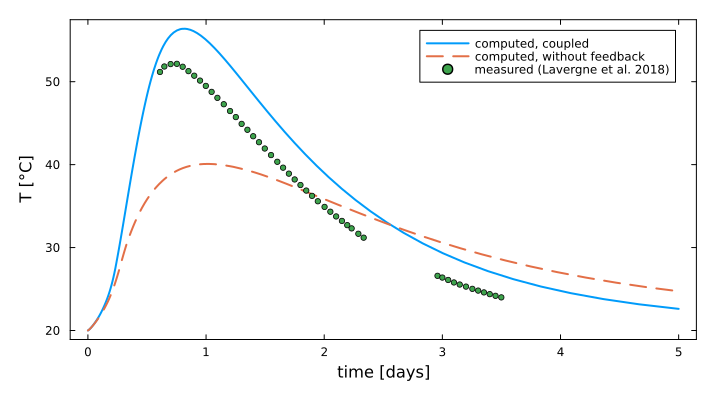

The coupled calculation reaches 56.4 °C at 0.81 day, where the measurement peaks at 52.1 °C at 0.75 day, and it stays 2.8 to 5.4 K above the measured curve through the cooling that follows. Nothing has been adjusted on this curve: the kinetic parameters are those of the model of the paste, the cell and its losses those Lavergne et al. (2018) calibrated. The run without feedback, the heat flow of the paste held at 20 °C integrated afterwards through the same cell, peaks at 40.1 °C only, and later, at 1.02 day. The difference, 16 K out of a rise of 36 K, is the acceleration of the reactions by the temperature they raise, through their activation energies; a semi-adiabatic test is therefore a test of those energies as much as of the heat, and it cannot be read off an isothermal calculation.

Limestone in place of cement

Lavergne et al. (2018), Fig. 15(a) runs the same test on four mortars where limestone replaces 5 to 30 % of the cement, at w/b = 0.5 (Table 11). The mixes differ by more than the filler: the binder of a mortar rises from 371 g without limestone to 503 to 566 g with it, and the sand falls, so that the measured maximum rises from 52.2 °C without limestone to 63.8 °C with 10 %, and falls back as the limestone grows. The model of the paste holds the limestone as calcite, which enters the chemistry, into carboaluminates, and not the rates: the kinetic law reads the fineness of the cement alone. Two of the four mortars, with 15 and 30 % of limestone, run here as the plain one did; the curves of the figure are a raster image, read where the band of each mortar is not covered by another (data/literature/Lavergne2018.json).

limestone = Dict(map(("C85L15", "C70L30")) do name
    m = calorimetry_mix(name)
    fc = parse(Int, match(r"^C(\d+)", name)[1]) / 100          # cement in the binder
    c = semiadiabatic_cell(; mix = m, T0 = T_env, T_env)
    r = quiet() do
        run_ionic_hydration(; wb = m.wb, binder_mass = m.binder, gypsum = fc * IONIC_CEMENT.gypsum,
                            filler = fc * IONIC_CEMENT.filler + (1 - fc), calorimeter = c,
                            tend = 3.5 * 86400.0)
    end
    name => temperature_profile(r.sol, c)
end)
limestone["C100"] = temperature_profile(semi.sol, cell)
# The measured temperature of a mortar: times in days, temperatures in °C.
lime = literature_table("Lavergne2018", "semi_adiabatic_limestone_wb050_temperature")
function measured_T(name)
    name == "C100" && return ustrip.(u"d", meas.time), meas.temperature_C
    i = findall(==(name), lime.mix)
    return ustrip.(u"d", lime.time[i]), lime.temperature_C[i]
end
peaks = literature_table("Lavergne2018", "semi_adiabatic_wb050_maximum")
println("mortar   maximum, measured     maximum, computed      at 2.5 days, measured  computed")
for (k, name) in enumerate(peaks.mix)
    measured = @sprintf("%5.1f °C at %.2f d", peaks.temperature_C[k], ustrip(u"d", peaks.time[k]))
    if haskey(limestone, name)
        t, T = limestone[name]
        j = argmax(T)
        tm, Tm = measured_T(name)
        @printf("%-7s  %s   %5.1f °C at %.2f d             %5.1f °C  %5.1f °C\n", name, measured,
                T[j] - 273.15, t[j] / 86400, interp(2.5, tm, Tm), interp(2.5 * 86400, t, T) - 273.15)
    else
        @printf("%-7s  %s   not run\n", name, measured)
    end
end

mortar   maximum, measured     maximum, computed      at 2.5 days, measured  computed
┌ Warning: Assignment to `t` in soft scope is ambiguous because a global variable by the same name exists: `t` will be treated as a new local. Disambiguate by using `local t` to suppress this warning or `global t` to assign to the existing global variable.
└ @ lavergne2018.md:680
┌ Warning: Assignment to `T` in soft scope is ambiguous because a global variable by the same name exists: `T` will be treated as a new local. Disambiguate by using `local T` to suppress this warning or `global T` to assign to the existing global variable.
└ @ lavergne2018.md:680
┌ Warning: Assignment to `j` in soft scope is ambiguous because a global variable by the same name exists: `j` will be treated as a new local. Disambiguate by using `local j` to suppress this warning or `global j` to assign to the existing global variable.
└ @ lavergne2018.md:681
┌ Warning: Assignment to `tm` in soft scope is ambiguous because a global variable by the same name exists: `tm` will be treated as a new local. Disambiguate by using `local tm` to suppress this warning or `global tm` to assign to the existing global variable.
└ @ lavergne2018.md:682
┌ Warning: Assignment to `Tm` in soft scope is ambiguous because a global variable by the same name exists: `Tm` will be treated as a new local. Disambiguate by using `local Tm` to suppress this warning or `global Tm` to assign to the existing global variable.
└ @ lavergne2018.md:682
C100      52.2 °C at 0.71 d    56.4 °C at 0.82 d              30.0 °C   33.3 °C
C95L05    63.1 °C at 0.69 d   not run
C90L10    63.8 °C at 0.67 d   not run
C85L15    61.7 °C at 0.70 d    63.9 °C at 0.81 d              35.1 °C   35.5 °C
C70L30    58.6 °C at 0.67 d    54.8 °C at 0.92 d              30.6 °C   34.6 °C
C95SF05   66.6 °C at 0.58 d   not run
C75FA25   60.4 °C at 0.78 d   not run
C50FA50   55.8 °C at 0.82 d   not run

p = plot(; xlabel = "time [days]", ylabel = "T [°C]", xlims = (0, 3.5), size = (720, 420),
         legend = :topright, title = "computed (lines), measured (markers)")
for (k, name) in enumerate(("C100", "C85L15", "C70L30"))
    col = palette(:tab10)[k]
    t, T = limestone[name]
    plot!(p, t ./ 86400, T .- 273.15; color = col, lw = 2, label = name)
    scatter!(p, measured_T(name)...; color = col, ms = 2.5, label = "")
end
p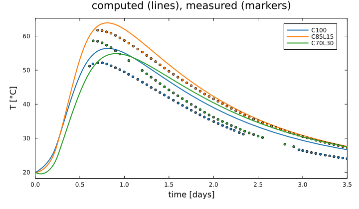

Without limestone and with 15 % of it, the calculation peaks 4.2 and 2.2 K above the measurement, some two and a half hours late. With 30 % it falls 3.8 K short, and late by nearly six hours: the measured maximum comes as early with 30 % of limestone as without, where the calculation, whose rates follow the cement alone, delays it as the cement is diluted. A filler that hastens the hydration of the cement would account for a peak both earlier and higher; the kinetic law, which reads the fineness of the cement alone, holds no such effect. Through the cooling, at two and a half days, the calculation stands 3.3, 0.4 and 4.0 K above the measurements of the plain mortar and of those with 15 and 30 % of limestone.

Silica fume in place of cement

Lavergne et al. (2018), Fig. 16(a) runs the test on mortars where silica fume replaces 5 and 15 % of the cement, and fly ash 25 and 50 %. The measured curves of the mortars with silica fume end near 0.7 day, that with 15 % before its maximum. The mortar with 5 % runs here over a day, with the fume of Table 7 as in the paste above. That with 15 % is not run, its integration taking more than forty minutes, nor those with fly ash, of which the article gives the class, F, and not the composition.

pozz = literature_table("Lavergne2018", "semi_adiabatic_pozzolan_wb050_temperature")
msf = calorimetry_mix("C95SF05")
csf = semiadiabatic_cell(; mix = msf, T0 = T_env, T_env)
rsf = quiet() do
    run_ionic_hydration(; wb = msf.wb, binder_mass = msf.binder, gypsum = 0.95 * IONIC_CEMENT.gypsum,
                        filler = 0.95 * IONIC_CEMENT.filler, silica_fume = lavergne_addition("SF", 0.05),
                        calorimeter = csf, tend = 86400.0)
end
tsf5, Tsf5 = temperature_profile(rsf.sol, csf)
j = argmax(Tsf5)
k = findfirst(==("C95SF05"), peaks.mix)
@printf("C95SF05: maximum measured %.1f °C at %.2f d, computed %.1f °C at %.2f d\n",
        peaks.temperature_C[k], ustrip(u"d", peaks.time[k]), Tsf5[j] - 273.15, tsf5[j] / 86400)
p = plot(; xlabel = "time [days]", ylabel = "T [°C]", xlims = (0, 1), size = (720, 420),
         legend = :topleft, title = "computed (lines), measured (markers)")
t, T = limestone["C100"]
plot!(p, t ./ 86400, T .- 273.15; color = palette(:tab10)[1], lw = 2, label = "C100")
scatter!(p, measured_T("C100")...; color = palette(:tab10)[1], ms = 2.5, label = "")
plot!(p, tsf5 ./ 86400, Tsf5 .- 273.15; color = palette(:tab10)[4], lw = 2, label = "C95SF05")
for (name, col) in (("C95SF05", 4), ("C85SF15", 5))
    i = findall(==(name), pozz.mix)
    scatter!(p, ustrip.(u"d", pozz.time[i]), pozz.temperature_C[i]; color = palette(:tab10)[col], ms = 2.5,
             label = name == "C85SF15" ? "C85SF15, measured" : "")
end
p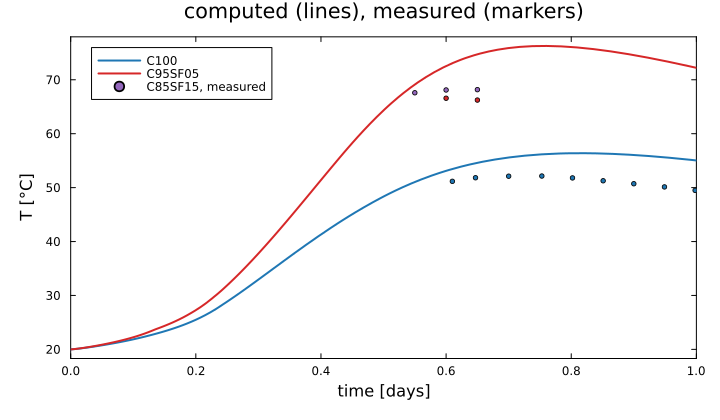

With 5 % of silica fume the calculation peaks at 76.3 °C at 0.75 day, 9.7 K above the measurement and four hours after it, 66.6 °C at 0.58 day. The law of the fume is that of a fly ash at five times its fineness, as the article sets it, with an activation energy of 83 kJ/mol, twice that of alite: as the cell warms, the fume reacts the faster, and its heat adds to that of the clinker in the same hours. The measured mortars with silica fume rise some 15 K above the plain one; the calculation puts 20 K between the plain mortar and that with 5 % of fume.

What this page does not reproduce yet

The bound water and the portlandite of the pastes of Pane and Hansen (2005) with silica fume and fly ash, Lavergne et al. (2018), Fig. 8, need the proportions of their blends, which the article does not give. The adiabatic concretes of Fig. 9(a) need their mixes, which are in the work of Waller (1999) and not in the article. Of the semi-adiabatic mortars, those with fly ash are left out, the article giving its class and not its composition, and so is that with 15 % of silica fume, whose integration takes more than forty minutes. The mortars at w/b = 0.32 of Figs. 15(b) and 16(b) are left out too, their curves covering one another in the raster images of the figures so that few can be read; at w/b = 0.5, the mortars with 5 and 10 % of limestone are read, their maxima printed above, and not run, each semi-adiabatic run costing minutes.

See also

• A complete CEM I 52.5 N, through its pore solution, the model of the paste and its assumptions.

• Hydration kinetics of a CEM I 52.5 R clinker, the same law on the stoichiometric formulation.

• CEM I 52.5 N and slag in an isothermal calorimeter, read off the states and Bound water of CEM I 52.5 N and slag pastes, and the thermogram it integrates to, the measurements that are outputs of a calculation rather than part of it.