
Validation against a measured paste: a CEM I 42.5 N through its first year
Before this page
A calculation is worth what it predicts about a paste that was measured. Lothenbach and Winnefeld (2006) hydrated a CEM I 42.5 N at a water/cement ratio of 0.5 and 20 °C, extracted its pore solution from the first minute to 317 days, analyzed it (their Table 3), and modeled the paste with a thermodynamic code fed by the dissolution rates of the clinker phases. This page repeats that calculation from the published data and compares it with what they measured.
Two comparisons are made, and they answer different questions:
against the measurement: is the model right about this paste?
against another code, GEMS3K run (Kulik et al., 2013) on the same budgets with the same phases: when the model is wrong, is it the model or ChemistryLab?
using ChemistryLab
using DynamicQuantities
using JSON
using Printf
using Plots
default(framestyle = :box, grid = false)

# The cement, its recipe and its system, shared with the test of this page and
# with the generator of the GEMS3K replay.
include(joinpath(pkgdir(ChemistryLab), "scripts", "lothenbach_winnefeld_2006.jl"))
model = cemdata18_activity_model(:KOH)
1. The cement
Lothenbach and Winnefeld (2006) give the composition as normative phases, computed from the chemical analysis (Table 1), and the sodium, potassium, magnesium and sulfate each clinker phase carries (Table 2). Those minor elements are released with their phase, as it dissolves; the alkali sulfates, the calcium sulfates, calcite and the free lime are available from the start.
cement = lw06_material()
for c in cement.constituents
    @printf("  %-24s %6.2f g per 100 g\n", c.name, 100c.mass_fraction)
end
alite 55.00 g per 100 g
alite minors 1.23 g per 100 g
belite 15.00 g per 100 g
belite minors 0.30 g per 100 g
aluminate 7.90 g per 100 g
aluminate minors 0.27 g per 100 g
ferrite 8.10 g per 100 g
ferrite minors 0.45 g per 100 g
free lime 0.46 g per 100 g
Cal 4.40 g per 100 g
Anh 2.50 g per 100 g
hemihydrate 0.50 g per 100 g
Gp 1.50 g per 100 g
K2SO4 1.60 g per 100 g
Na2SO4 0.10 g per 100 g
SrO 0.07 g per 100 g2. How much has reacted
Each clinker phase dissolves by the rate law of Parrott and Killoh (1984), with the parameters of Table 4 and the correction the paper applies for the water/cement ratio: past a degree of hydration of 1.333 w/c, the rate is multiplied by
println("            1 d     28 d    317 d")
for c in cement.constituents
    c isa MineralConstituent && c.extent isa ParrottKillohExtent || continue
    @printf("  %-9s %6.3f  %6.3f  %6.3f\n", c.name, (extent(c.extent, t) for t in (1, 28, 317))...)
end
1 d 28 d 317 d
alite 0.369 0.766 0.838
belite 0.114 0.518 0.718
aluminate 0.346 0.767 0.839
ferrite 0.152 0.690 0.7963. The paste at each age of the measurement
The system holds the clinker phases, the calcium sulfates, the hydrates of the assemblage of Lothenbach and Winnefeld (2006) and the C-S-H as the CSHQ model of Cemdata18 (Lothenbach et al., 2019), whose end-members KSiOH and NaSiOH take up alkalis. The paste is solved at each age of Table 3, each age started from the one before:
cs = lw06_system()
hours = lw06_hours()
states = hydrate(lw06_recipe(), cs, hours ./ 24; model)
@printf("%d ages from %.2f h to %.0f days\n", length(hours), first(hours), last(hours) / 24)
16 ages from 0.02 h to 317 days4. The pore solution, against the measurement
The model gives millimoles per kilogram of water, the analysis millimoles per liter of solution; the two differ by the density of the solution and the mass of its solutes, a few percent at these concentrations, which is small beside most of the differences below. A value Lothenbach and Winnefeld (2006) give only as a detection limit is printed <x and not plotted.
elements = ["K", "Na", "Ca", "S", "Si", "Al", "OH-"]
model_at = [lw06_pore_solution(rs.state) for rs in states]
println("   age        ", join((rpad(e, 16) for e in elements)))
println("              ", join((rpad("model/measured", 16) for _ in elements)))
for (k, h) in enumerate(hours)
    h in (1.0, 16.0, 26.0, 144.0, 696.0, 7608.0) || continue
    @printf("%9.1f h   ", h)
    for e in elements
        m = lw06_measured(h, e)
        print(rpad(@sprintf("%.3g/%s%.3g", model_at[k][e], m.below_limit ? "<" : "", m.value), 16))
    end
    println()
end
age K Na Ca S Si Al OH-
model/measured model/measured model/measured model/measured model/measured model/measured model/measured
1.0 h 378/360 27.5/28 13/22.2 161/156 0.0312/0.09 7.85e-07/0.03 101/130
16.0 h 441/430 24.7/32 12.5/9.5 188/136 0.0311/0.07 8.32e-07/<0.004 105/200
26.0 h 411/430 14.4/44 1.43/4.2 47.4/83 0.0534/0.17 0.000458/<0.007 312/360
144.0 h 400/520 8.03/55 0.968/2.1 3.26/10 0.0639/0.24 0.0531/0.09 379/520
696.0 h 405/560 6.65/63 0.956/1.2 3.34/11 0.0647/0.27 0.0537/0.12 382/540
7608.0 h 407/640 5.78/65 0.954/1.5 3.36/16 0.0649/0.21 0.0538/0.11 383/590panels = map(("K", "Na", "Ca", "S", "Si", "OH-")) do e
p = plot(; xscale = :log10, yscale = :log10, title = e, xlabel = "time (h)",
ylabel = "mmol/kg or mmol/L", legend = e == "K" ? :bottomright : false)
plot!(p, hours, [m[e] for m in model_at]; label = "ChemistryLab", color = :steelblue, linewidth = 2)
measured = [lw06_measured(h, e) for h in hours]
scatter!(p, hours, [m.below_limit ? NaN : m.value for m in measured]; label = "measured", color = :black)
p
end
fig = plot(panels...; layout = (2, 3), size = (900, 560),
left_margin = 6Plots.mm, bottom_margin = 6Plots.mm)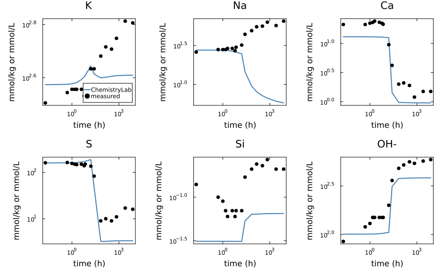
Where the alkalis are at the last age, between the C-S-H and the solution:
final = states[end].state
n = ustrip.(us"mol", final.n)
total(el) = sum(get(atoms(sp), el, 0) * x for (sp, x) in zip(final.system.species, n))
gel = solid_solution_totals(final, "CSHQ").elements
for el in (:K, :Na)
    @printf("at 317 days the C-S-H holds %.0f %% of the %s\n", 100gel[el] / total(el), el === :K ? "potassium" : "sodium")
end
at 317 days the C-S-H holds 68 % of the potassium
at 317 days the C-S-H holds 96 % of the sodium5. The same budgets through GEMS3K
test/reference/xgems_lw2006.json holds the answer of GEMS3K on the budget of each age, with the phases of this system and the extended Debye–Hückel model of Cemdata18; the xGEMS export it runs on is the Cemdata18 cement of that repository. The file was written by running the code, and the test suite checks this page's paste against it.
fixture = JSON.parsefile(joinpath(pkgdir(ChemistryLab), "test", "reference", "xgems_lw2006.json"))
answered = count(row -> row["converged"], fixture["rows"])
worst = Dict(e => 0.0 for e in elements)
worst_pH = 0.0
for (k, row) in enumerate(fixture["rows"])
    row["converged"] || continue
    gems = row["mmol_per_kg_water"]
    for e in elements
        worst[e] = max(worst[e], abs(model_at[k][e] / gems[e] - 1))
    end
    global worst_pH = max(worst_pH, abs(pH(states[k].state, model) - row["pH"]))
end
@printf("compared at the %d of the %d ages the reference file holds an answer for\n", answered, length(fixture["rows"]))
@printf("largest difference in pH over the ages: %.4f\n", worst_pH)
for e in elements
    @printf("  %-4s largest relative difference: %.2f %%\n", e, 100worst[e])
end
compared at the 15 of the 16 ages the reference file holds an answer for
largest difference in pH over the ages: 0.0008
K largest relative difference: 0.09 %
Na largest relative difference: 0.12 %
Ca largest relative difference: 0.22 %
S largest relative difference: 0.66 %
Si largest relative difference: 1.62 %
Al largest relative difference: 0.64 %
OH- largest relative difference: 0.08 %6. What the comparison says
The two codes agree. On the fifteen ages of the reference, the two answers differ by less than 0.001 in pH, by 1.6 % on silicon and by less than 0.7 % on every other element. What separates the calculation from the paste is therefore a property of the model, of the database and of the assumptions of section 3, and it would be found with either code.
The first day is reproduced where an equilibrium can reproduce it. Potassium is within 5 % of the measurement at 1 and 16 h, sodium and sulfate at 1 h. The consumption of the calcium sulfates between 16 and 26 h shows in both: the sulfate falls and the hydroxide rises, from 105 to 312 mmol/kg in the model and from 200 to 360 mmol/L in the paste. The calcium is 40 % low in the first hours, 13 against 22 mmol; Lothenbach and Winnefeld (2006) note that the early solutions are oversaturated with respect to portlandite, gypsum, ettringite and syngenite, the clinker releasing calcium faster than those solids precipitate, and an equilibrium cannot represent an oversaturated solution.
The alkalis are where the model departs. From the second day on, the model's potassium stays near 400 mmol/kg while the measured one rises to 640 by 317 days, and its sodium falls to 6 mmol/kg while the measurement rises to 65, a tenth of it. The hydroxide, which balances the alkalis, is a third low. Both come from the C-S-H: CSHQ takes the alkalis up through its KSiOH and NaSiOH end-members, and at 317 days it holds 68 % of the potassium and 96 % of the sodium. The authors modeled that uptake differently, as a distribution ratio of 0.42 mL per gram of C-S-H for both alkalis, the mean Hong and Glasser (1999) measured at a C/S of 1.8. This is where the calculation, run with the C-S-H model Cemdata18 ships, departs from theirs, and from the paste.
Silicon, aluminum and the late sulfate are low by factors of 2 to 5: silicon 0.065 against 0.21 to 0.27 mmol, aluminum 0.054 against 0.09 to 0.12, sulfate 3.4 against 10 to 16 from the sixth day. These are the concentrations the solubilities of the C-S-H and of the aluminate hydrates of the database fix, and both codes give the same.
For a user, the page draws the line this way: the hydroxide within a third and the potassium of the first day are what the model gives this cement; the sodium and the minor elements depend on a C-S-H whose alkali uptake is stronger than the paste shows, and a calculation that needs them should say which uptake it assumes.
Where to go next
The recipe layer this page is built on is described in Recipes: materials, extents and what has not reacted, and the C-S-H models of the package in The models of the C-S-H gel.