
A published clay sorption model
Before this page
Two families of sites, and a metal between them, and Chemistry that happens on a surface §7 for cation exchange.
Every surface example so far was built here, from constants chosen to make a point. This one is somebody else's model, read out of the file its authors published (Marinich et al., 2025), and run against the code they published it for.
ClaySor 2023 (Marinich et al., 2025) is the 2SPNE SC/CE model of Bradbury and Baeyens for illite and montmorillonite: two-site protolysis, non-electrostatic, plus cation exchange. It is a good test of this package for a reason beyond its constants — a clay carries four site budgets on one solid, three edge families and an exchanger, and they compete for the same solution.
What this is not
ClaySor's constants were fitted against the PSI/Nagra TDB 2020 aqueous database. This repository does not have it. Both sides of the comparison below therefore run the ClaySor sorption model over phreeqc.dat's aqueous chemistry, which tests the implementation of the model and is not a reproduction of ClaySor. Using its constants over a different aqueous database is a different model, in the same way a surface constant fitted with a diffuse layer is a different constant from one fitted without.
The constants are read, not retyped
using ChemistryLab, DynamicQuantities, SciMLBase, OptimaSolver, JSON, Printf

CS = JSON.parsefile(joinpath(pkgdir(ChemistryLab), "test", "reference",
                             "phreeqc_claysor.json"))
println(CS["model"])
println(CS["model_file"], "  doi:", CS["model_doi"], "  ", CS["model_licence"])
for r in CS["reactions"]["surface"][1:2]
    @printf("  %-34s log K %6.2f   %s\n", r["equation"], r["log_K"],
            something(r["reference"], "—"))
end
for r in CS["reactions"]["exchange"]
    @printf("  %-34s log K %6.3f   %s\n", r["equation"], r["log_K"],
            something(r["reference"], "—"))
end
ClaySor 2023 (2SPNE SC/CE), Na-montmorillonite subset
claysor23_v0.7.dat doi:10.5281/zenodo.15095062 CC-BY-4.0
H+ + Mnt_sOH = Mnt_sOH2+ log K 4.50 Bradbury_Baeyens:1997:pap:
Mnt_sOH = Mnt_sO- + H+ log K -7.90 Bradbury_Baeyens:1997:pap:
Mntx- + Na+ = MntxNa log K 0.000 —
Ca+2 + 2 MntxNa = Mntx2Ca + 2 Na+ log K 0.396 Curti:2023:rep:read_sorption_model is what produced those, straight from claysor23_v0.7.dat, and it keeps what travels with each constant: the ref: tag becomes the Traced source and the error: tag its uncertainty. Over the whole compilation that is 187 reactions, all published — and 60 of them state no uncertainty at all, which provenance_report says in one line and which reading the numbers never would.
Four budgets on one clay
The three edge families become pseudo-elements Xs, Xv, Xw, and the exchanger Xm. ClaySor's own names cannot be used as written: Mnt_sOH would be read as chemistry, which is exactly the trap the reserved site symbols exist to avoid.
The exchanger mixes in the Gaines-Thomas convention, because that is what PHREEQC's EXCHANGE block uses (Parkhurst and Appelo, 2013); the edge families mix ideally, because the model is non-electrostatic by construction — the NE of 2SPNE.
sites = CS["sites_mol_per_g"]
@printf("edge sites   strong %.1e   weak-1 %.1e   weak-2 %.1e  mol/g\n",
        sites["Mnt_sOH"], sites["Mnt_vOH"], sites["Mnt_wOH"])
@printf("exchanger    CEC %.5f mol/g of charge\n", CS["cec_mol_per_g"])
@printf("surface      %.0f m²/g\n", CS["specific_area_m2_per_g"])
edge sites strong 2.0e-06 weak-1 4.0e-05 weak-2 4.0e-05 mol/g
exchanger CEC 0.00087 mol/g of charge
surface 18 m²/gThose four numbers are documented in ClaySor's own header for 1 g of Na-montmorillonite, which is where they come from here.
Against PHREEQC
The system below is the one test/claysor.jl builds and checks, written out: the aqueous species from slop98, the surface species built from the constants read above, one support of 1 g of clay for the four families.
using SciMLBase, Plots
const SLOP = Dict(symbol(s) => s for s in build_species(datapath("slop98-inorganic-thermofun.json"); verbose = false))
h2o, hp, oh, na, ca, cl = (SLOP[s] for s in ("H2O@", "H+", "OH-", "Na+", "Ca+2", "Cl-"))
RT = R_GAS * 298.15
G(s) = ustrip(us"J/mol", s[:ΔₐG⁰](T = 298.15u"K", P = 1.0e5u"Pa"; unit = true))
# The log K of the reaction that produces `species`, read from the fixture.
logK(species) = first(r["log_K"] for r in vcat(CS["reactions"]["surface"], CS["reactions"]["exchange"])
                       if occursin(species, split(r["equation"], "=")[2]))
function surface_species(sym, g)
    s = Species(sym; aggregate_state = AS_SURFACE, class = SC_SURFCOMPLEX)
    s[:ΔₐG⁰] = SymbolicFunc(g * u"J/mol")
    return s
end

function clay(chloride)
    support = SurfaceSupport("Na-montmorillonite", nothing, BETSurfaceArea(CS["specific_area_m2_per_g"] * 1000.0))
    families, species, masters = SiteFamily[], Any[h2o, hp, oh, na, ca, cl], Any[]
    for (sym, phreeqc) in (("Xs", "Mnt_s"), ("Xv", "Mnt_v"), ("Xw", "Mnt_w"))
        free = surface_species("$(sym)OH", 0.0)
        prot = surface_species("$(sym)OH2+", -RT * log(10) * logK("$(phreeqc)OH2+"))
        depr = surface_species("$(sym)O-", -RT * log(10) * logK("$(phreeqc)O-"))
        capacity = TotalSiteAmount(sites["$(phreeqc)OH"] * CS["grams"])
        push!(families, SiteFamily(phreeqc, free, [prot, depr]; capacity, support))
        append!(species, (free, prot, depr))
        push!(masters, free)
    end
    # The exchanger, in the Gaines-Thomas convention of PHREEQC's EXCHANGE.
    naX = surface_species("NaXm", 0.0)
    caX = surface_species("CaXm2", -RT * log(10) * logK("Mntx2Ca") + G(ca) - 2G(na))
    push!(families, SiteFamily("Mntx", naX, [caX]; capacity = TotalSiteAmount(CS["cec_mol_per_g"] * CS["grams"]),
                               support, model = GainesThomasMixing()))
    append!(species, (naX, caX))
    cs = ChemicalSystem(identity.(species), identity.(vcat([h2o, hp, na, ca, cl], masters, [naX]));
                        site_families = identity.(families))
    idx = Dict(symbol(sp) => k for (k, sp) in enumerate(cs.species))
    n = Any[fill(1.0e-14u"mol", length(cs.species))...]
    n[idx["H2O@"]] = 1.0u"kg" / h2o[:M]
    n[idx["Na+"]], n[idx["Ca+2"]], n[idx["Cl-"]] = CS["na"] * u"mol", CS["ca"] * u"mol", chloride * u"mol"
    for (sym, phreeqc) in (("Xs", "Mnt_s"), ("Xv", "Mnt_v"), ("Xw", "Mnt_w"))
        n[idx["$(sym)OH"]] = sites["$(phreeqc)OH"] * CS["grams"] * u"mol"
    end
    n[idx["NaXm"]] = CS["cec_mol_per_g"] * CS["grams"] * u"mol"
    return cs, ChemicalState(cs, n), idx
end

# Each point at the pH and the ionic strength of PHREEQC's, the chloride
# carrying the difference its titrant made.
function solve_point(pt, model)
    mH, mOH = 10.0^(-pt["pH"]), 10.0^(pt["pH"] - 14)
    cs, st, idx = clay(2pt["I"] - CS["na"] - 4CS["ca"] - mH - mOH)
    des = DualEquilibriumSolver(cs, model)
    b = budget(st)
    eq = SciMLBase.solve(des, st; b, constraint = FixedpH(pt["pH"]), parameters = Base.RefValue{Any}(nothing))
    cert = optimality_certificate(des, eq; b, constraint = FixedpH(pt["pH"]))
    n = Float64[ustrip(us"mol", x) for x in eq.n]
    return (; certified = cert.stationarity < 1.0e-8, n = s -> n[idx[s]])
end
ours = [solve_point(pt, DaviesActivityModel()) for pt in CS["points"]]
println("certified: ", count(r -> r.certified, ours), " of ", length(ours))

using Markdown
rows = ["| pH | NaX, ours | NaX, PHREEQC | ≡XsO⁻, ours | ≡XsO⁻, PHREEQC |",
        "|---:|---:|---:|---:|---:|"]
for (pt, r) in zip(CS["points"], ours)
    s = pt["species"]
    push!(rows, @sprintf("| %.1f | %.4e | %.4e | %.4e | %.4e |",
                         pt["pH"], r.n("NaXm"), s["MntxNa"], r.n("XsO-"), s["Mnt_sO-"]))
end
Markdown.parse(join(rows, "\n"))| pH | NaX, ours | NaX, PHREEQC | ≡XsO⁻, ours | ≡XsO⁻, PHREEQC |
|---|---|---|---|---|
| 4.0 | 5.8623e-04 | 5.8059e-04 | 6.0490e-11 | 6.0490e-11 |
| 5.0 | 5.8621e-04 | 5.8057e-04 | 1.9111e-09 | 1.9111e-09 |
| 6.0 | 5.8620e-04 | 5.8056e-04 | 2.4112e-08 | 2.4112e-08 |
| 7.0 | 5.8620e-04 | 5.8056e-04 | 2.2301e-07 | 2.2301e-07 |
| 8.0 | 5.8620e-04 | 5.8056e-04 | 1.1145e-06 | 1.1145e-06 |
| 9.0 | 5.8620e-04 | 5.8057e-04 | 1.8528e-06 | 1.8528e-06 |
| 10.0 | 5.8620e-04 | 5.8067e-04 | 1.9842e-06 | 1.9842e-06 |
The strong sites and the exchanger across the pH range, ours as lines and PHREEQC's as markers:
pHs = [pt["pH"] for pt in CS["points"]]
N_s = sites["Mnt_sOH"] * CS["grams"]
p_edge = plot(; xlabel = "pH", ylabel = "fraction of the strong sites", legend = :right,
              title = @sprintf("Strong sites, %.0e mol/g", sites["Mnt_sOH"]), titlefontsize = 10)
for (k, (o, t, lab)) in enumerate((("XsOH2+", "Mnt_sOH2+", "≡SOH₂⁺"), ("XsOH", "Mnt_sOH", "≡SOH"), ("XsO-", "Mnt_sO-", "≡SO⁻")))
    plot!(p_edge, pHs, [r.n(o) / N_s for r in ours]; lw = 2, color = k, label = lab)
    scatter!(p_edge, pHs, [pt["species"][t] / N_s for pt in CS["points"]]; color = k, marker = :diamond, label = "")
end
cec = CS["cec_mol_per_g"] * CS["grams"]
p_ex = plot(pHs, [2r.n("CaXm2") / cec for r in ours]; lw = 2, color = 1, label = "Ca, ours", ylims = (0, 1),
            xlabel = "pH", ylabel = "equivalent fraction of the CEC", legend = :right,
            title = @sprintf("Exchanger, CEC %.5f mol/g", CS["cec_mol_per_g"]), titlefontsize = 10)
scatter!(p_ex, pHs, [2pt["species"]["Mntx2Ca"] / cec for pt in CS["points"]]; color = 1, marker = :diamond, label = "Ca, PHREEQC")
plot!(p_ex, pHs, [r.n("NaXm") / cec for r in ours]; lw = 2, color = 2, label = "Na, ours")
scatter!(p_ex, pHs, [pt["species"]["MntxNa"] / cec for pt in CS["points"]]; color = 2, marker = :diamond, label = "Na, PHREEQC")
plot(p_edge, p_ex; layout = (1, 2), size = (960, 380), left_margin = 6Plots.mm, bottom_margin = 6Plots.mm)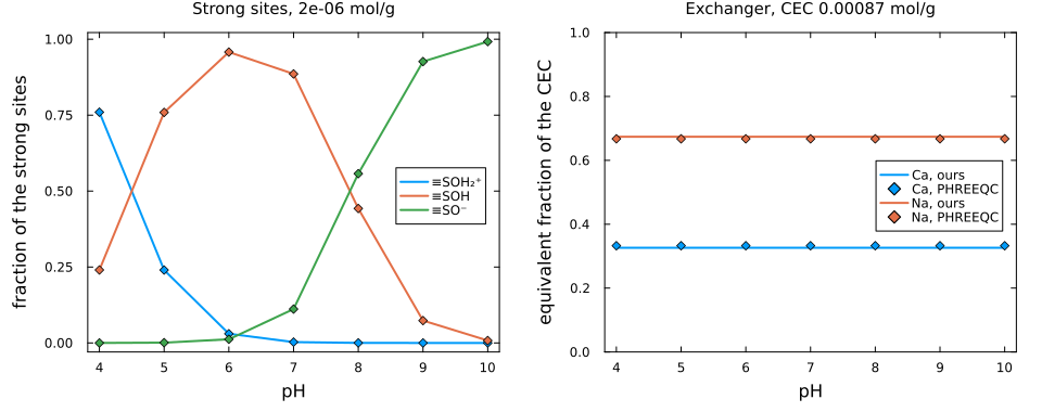
And the worst relative gaps over the seven points, with the gap on the exchanger at pH 7 under ideal activities beside it:
gap(r, pt, pairs) = maximum(abs(r.n(o) / pt["species"][t] - 1) for (o, t) in pairs if pt["species"][t] > 1.0e-12)
edge_pairs = (("XsOH", "Mnt_sOH"), ("XsOH2+", "Mnt_sOH2+"), ("XsO-", "Mnt_sO-"), ("XwOH", "Mnt_wOH"), ("XwO-", "Mnt_wO-"))
exchange_pairs = (("NaXm", "MntxNa"), ("CaXm2", "Mntx2Ca"))
@printf("edge sites %.1e, exchanger %.1e (Davies)\n",
        maximum(gap(r, pt, edge_pairs) for (r, pt) in zip(ours, CS["points"])),
        maximum(gap(r, pt, exchange_pairs) for (r, pt) in zip(ours, CS["points"])))
pt7 = CS["points"][4]
@printf("exchanger at pH %.0f: %.1f %% ideal, %.2f %% Davies\n", pt7["pH"],
        100gap(solve_point(pt7, DiluteSolutionModel()), pt7, exchange_pairs), 100gap(ours[4], pt7, exchange_pairs))
edge sites 2.5e-06, exchanger 2.0e-02 (Davies)
exchanger at pH 7: 23.8 % ideal, 1.95 % DaviesThe edge sites agree to 2.5 × 10⁻⁶ and the exchanger to 2.0 × 10⁻², four orders of magnitude apart, and the reason is structural rather than accidental. The edge sites see only the proton, whose activity FixedpH prescribes on both sides, so no aqueous activity model enters and what is compared is the surface model alone. The exchanger sees the sodium and calcium activities, where Davies (Davies, 1962) and PHREEQC's extended Debye-Hückel genuinely differ.
That second sentence is a measurement, not an explanation offered after the fact: the identical system under ideal activities misses the exchanger at pH 7 by 23.8 %, against 1.95 % under Davies, the last line above. A factor of twelve from changing nothing but what the solution does — the same attribution, by the same protocol, as the zinc edge.
What it settles
A published sorption model, read from its own file rather than transcribed, reproduces here to 2.5 × 10⁻⁶ on the part where the comparison is of the surface model alone.
Four site budgets on one solid, three counting particles and one counting charge equivalents, close simultaneously and compete correctly.
And what is not settled is stated in the fixture itself, as a field: without PSI/Nagra TDB 2020 this is the model over a different aqueous chemistry, and calling it a reproduction would be claiming more than was checked.
See also
Cation exchange §7 — the two conventions and why one of them has to be declared rather than guessed.
Two families of sites, and a metal between them — the same machinery on an oxide, with the same attribution protocol.
Where the numbers come from — including
Traced, which is what carries a published constant's reference and uncertainty into the calculation.