
Bound water of CEM I 52.5 N and slag pastes, and the thermogram it integrates to
Before this page
CEM I 52.5 N and slag in an isothermal calorimeter, read off the states, which builds the same pastes.
A thermobalance weighs a dried sample while heating it. Between the drying temperature and the end of the run, the loss is the water the hydrates held and the carbon dioxide the carbonates held; the first, per gram of binder, is the bound water
What leaves, and how much
The plain paste at 28 months, the cement at the 74 % the image analysis gives, built by scripts/gruyaert2010.jl as on the calorimetry page.
using ChemistryLab, DynamicQuantities, Printf, Plots
include(joinpath(pkgdir(ChemistryLab), "scripts", "gruyaert2010.jl"))

cs = gruyaert_system()
G10(table, column; where...) = only(getproperty(literature_table("Gruyaert2010", table; where...), column))
αc(days, sb) = G10("hydration_degree", :alpha_cement; age_days = days * u"d", slag_to_binder = sb) / 100
αs(days, sb) = sb == 0 ? 0.0 :
    G10("hydration_degree_slag", :alpha_slag; age_days = days * u"d", slag_to_binder = sb) / 100
paste(days, sb) = gruyaert_paste(cs; slag = sb, alpha_cement = αc(days, sb), alpha_slag = αs(days, sb))

opc = paste(852, 0.0)
g(q) = ustrip(uconvert(us"g", q))
loss = ignition_loss(opc.eq)
@printf("certified %s; water %.2f g, CO2 %.2f g per 100 g of binder\n",
        opc.certificate.optimal, g(loss.water), g(loss.carbon_dioxide))
certified true; water 28.00 g, CO2 0.70 g per 100 g of binderignition_loss counts hydrogen, not formula water. Portlandite is Ca(OH)₂, has no H₂O written in it, and loses one per formula unit; a rule that searched the formula for H₂O would report none for it. Per phase:
for (ph, m) in bound_water_per_phase(opc.eq)                 # largest first
    g(m) > 0.05 && @printf("  %-15s %5.2f g\n", ph, g(m))
end
per_phase = [(ph, g(m)) for (ph, m) in bound_water_per_phase(opc.eq) if g(m) > 0.05]
p_w = bar(first.(per_phase), last.(per_phase); legend = false, color = :steelblue, xrotation = 30,
    ylabel = "g of water per 100 g of binder", size = (760, 380), left_margin = 6Plots.mm, bottom_margin = 12Plots.mm,
    title = "The plain paste at 28 months, cement 74 % hydrated, w/b 0.5")
plot!(p_w; ylims = (0, 1.1 * ylims(p_w)[2]))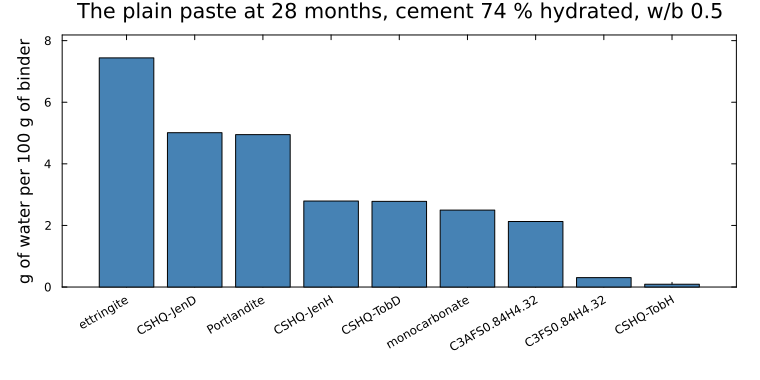
Against the thermobalance
The four pastes at the degrees of hydration of the image analysis, and the bound water of (Gruyaert et al., 2010; Fig. 7) at the nearest age, from the batch whose composition is that of the calorimetry (TG/b of Table 1). The image analysis is at 28 months and the thermogravimetry at 1018 days for the pastes with 0 and 50 % slag, at 363 days for the one with 85 %; the extrapolation to infinite time the article fits on each series,
wb_measured(sb, days) = only(literature_table("Gruyaert2010", "bound_water";
    batch = "b", slag_to_binder = sb, age_days = days * u"d").bound_water)
wb_inf(sb) = G10("bound_water_infinity", :bound_water_infinity; slag_to_binder = sb)
rows = [(2, 0.0, 1.997), (852, 0.0, 1018.264), (852, 0.5, 1018.264), (852, 0.85, 363.392)]
compared = []
println("  age  s/b    αc    αs   computed (ettringite)  measured (age)   w_b,∞")
for (days, sb, tg) in rows
    p = paste(days, sb)
    p.certificate.optimal || error("uncertified paste")
    aft = g(get(Dict(bound_water_per_phase(p.eq)), "ettringite", 0.0u"kg"))
    push!(compared, (; days, sb, computed = g(bound_water(p.eq)), measured = wb_measured(sb, tg),
                     infinity = days == 2 ? NaN : wb_inf(sb)))
    @printf("%5d  %4.2f  %4.2f  %4.2f   %6.2f  (%5.2f)      %6.2f (%4.0f d)   %s\n", days, sb,
            αc(days, sb), αs(days, sb), g(bound_water(p.eq)), aft, wb_measured(sb, tg), tg,
            days == 2 ? "  —" : @sprintf("%5.1f", wb_inf(sb)))
end
age s/b αc αs computed (ettringite) measured (age) w_b,∞
2 0.00 0.54 0.00 21.75 ( 7.44) 11.06 ( 2 d) —
852 0.00 0.74 0.00 28.00 ( 7.44) 21.43 (1018 d) 23.8
852 0.50 0.94 0.72 31.56 ( 2.02) 20.19 (1018 d) 22.4
852 0.85 0.91 0.39 18.65 ( 2.47) 11.49 ( 363 d) 11.4cases = [@sprintf("%s, %d %% slag", c.days == 2 ? "2 days" : "28 months", round(Int, 100c.sb)) for c in compared]
xs = collect(eachindex(cases))
fig = bar(xs .- 0.27, [c.computed for c in compared]; bar_width = 0.27, label = "computed: every hydrogen of the solids",
color = :steelblue, xticks = (xs, cases), ylabel = "bound water (g per 100 g of binder)", legend = :topleft,
size = (860, 420), left_margin = 6Plots.mm, bottom_margin = 6Plots.mm,
title = "At the degrees of the image analysis")
bar!(fig, xs, [c.measured for c in compared]; bar_width = 0.27, label = "thermobalance, above 105 °C", color = :black)
bar!(fig, xs .+ 0.27, [c.infinity for c in compared]; bar_width = 0.27, label = "w_b,∞ of the article", color = :grey60)
plot!(fig; ylims = (0, 1.2 * ylims(fig)[2]))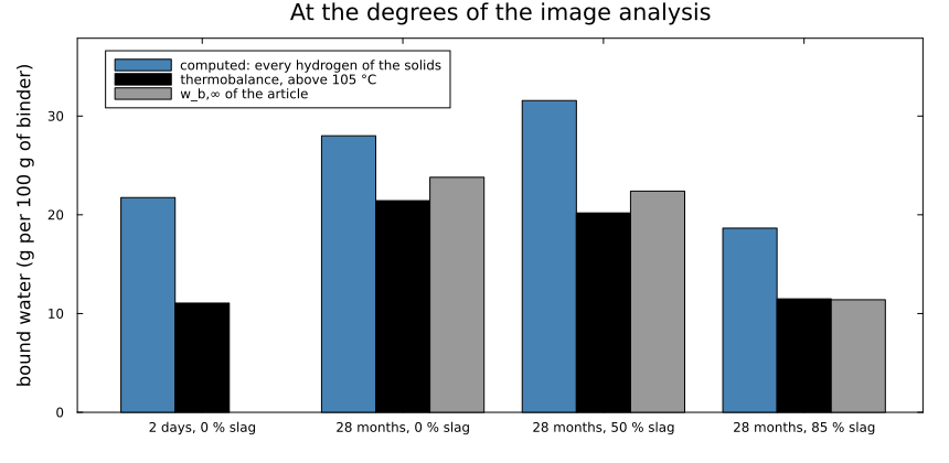
The calculation counts every hydrogen of the solids, the thermobalance only what leaves above 105 °C once the sample has been dried, so that the computed water is the larger in the four pastes, by 6.6 to 11.4 g per 100 g of binder, and the gap is not a constant fraction of it: the ratio is 2.0 at 2 days, 1.3 for the plain paste at 28 months and 1.6 for the two blends. In the plain paste the ettringite, which holds all the sulfate at both ages, carries 7.4 g of the computed water; in the blends it carries about 2 g, and the gap lies in the other hydrates. The drop at 85 % slag is found, from 31.6 to 18.7 g where the measurement goes from 20.2 to 11.5 g, whereas the order of the plain paste and of the blend with half slag is not: the blend holds more water than the plain paste in the calculation and less in the measurement. Which part of the water of each hydrate leaves before 105 °C is what a decomposition window per phase would state, and none is published for these pastes; the section below shows how such windows are identified from a measured curve, and what a curve cannot separate.
The shape of the curve, as a method
A total is not a thermogram. The curve needs to know when each phase goes, which is not a consequence of a formula; it comes from a publication or from a measurement, and DecompositionWindow makes a curve say which. This section is a self-test of that machinery on a mixture of portlandite, gypsum and calcite, with windows that are neither published nor measured: the target curve below is the model's own output, and nothing in it is a measurement.
using ChemistryLab, DynamicQuantities, Printf

c18 = Dict(symbol(s) => s for s in
           build_species(datapath("cemdata18-thermofun.json"); verbose = false))
aq = Dict(symbol(s) => s for s in
          build_species(datapath("slop98-inorganic-thermofun.json"); verbose = false))

cs = ChemicalSystem(
    vcat([aq[k] for k in ("H2O@", "H+", "Ca+2", "SO4-2", "CO3-2")],
         [c18[k] for k in ("Portlandite", "Gp", "Cal")]),
    [aq[k] for k in ("H2O@", "H+", "Ca+2", "SO4-2", "CO3-2")],
)
i = Dict(symbol(sp) => k for (k, sp) in enumerate(cs.species))
n = Any[fill(1.0e-12u"mol", length(cs.species))...]
n[i["H2O@"]] = ustrip(us"mol", 1.0u"kg" / aq["H2O@"][:M]) * u"mol"
n[i["Portlandite"]] = 1.0u"mol"; n[i["Gp"]] = 2.0u"mol"; n[i["Cal"]] = 3.0u"mol"
state = ChemicalState(cs, n)
loss = ignition_loss(state);
(water = 0.090074999968872 kg, carbon_dioxide = 0.13202699995437428 kg, total = 0.22210199992324628 kg)placeholder(phase, T½, w; releases = :water) = DecompositionWindow(
phase, T½, w; releases,
kind = PROV_PLACEHOLDER, source = "illustrative, not measured",
)
windows = [
placeholder("Gp", 400.0, 15.0),
placeholder("Portlandite", 720.0, 12.0),
placeholder("Cal", 950.0, 20.0; releases = :carbon_dioxide),
]
provenance_report([w.midpoint for w in windows])(total = 3, counts = Dict{ProvenanceKind, Int64}(PROV_UNSTATED => 0, PROV_ESTIMATED => 0, PROV_FITTED => 0, PROV_PLACEHOLDER => 3, PROV_PUBLISHED => 0, PROV_MEASURED => 0), weakest = PROV_PLACEHOLDER, all_evidence = false, without_uncertainty = 3)weakest = PROV_PLACEHOLDER is the report doing its job: whatever comes out of a calculation resting on these is a picture, not a measurement.
grid = range(300.0, 1200.0; length = 451)
tg = thermogram(state, windows; temperatures = grid)
@printf("starts at %7.3f g, ends at %7.3f g, loses %7.3f g (ignition_loss says %7.3f)\n",
        ustrip(uconvert(us"g", tg.mass[1] * us"kg")), ustrip(uconvert(us"g", tg.mass[end] * us"kg")),
        ustrip(uconvert(us"g", tg.loss[end] * us"kg")), ustrip(uconvert(us"g", loss.total)))
starts at 718.586 g, ends at 496.576 g, loses 222.102 g (ignition_loss says 222.102)The curve integrates to what the formulas say, which is the first thing to check and the one a wrong window silently breaks.
A phase with no window never leaves
It contributes to the starting mass and stays there, so a curve computed without noticing integrates to less than ignition_loss — and says nothing about it. phases_without_windows is how to see it — reporting phase => product, because a carbonated hydrate needs two windows and counting per phase would call it covered when half of it is.
phases_without_windows(state, windows[1:2]) # calcite left out1-element Vector{Pair{String, Symbol}}:
"Cal" => :carbon_dioxideThe curve and its derivative, each window drawn on its own:
using Plots
p_m = plot(grid, tg.mass_percent; lw = 2, color = :black, legend = false, xlabel = "temperature (K)",
           ylabel = "mass (% of initial)", title = "1 mol CH, 2 mol gypsum, 3 mol calcite", titlefontsize = 10)
vline!(p_m, [400.0, 720.0, 950.0]; ls = :dot, color = :grey50)
p_d = plot(; xlabel = "temperature (K)", ylabel = "−dm/dT (g per K)", title = "Its derivative, which resolves the phases",
           titlefontsize = 10, legend = :topleft)
for (w, lab, c) in zip(windows, ("gypsum", "portlandite", "calcite"), (:steelblue, :firebrick, :seagreen))
    plot!(p_d, grid, 1000 .* thermogram(state, [w]; temperatures = grid).dtg; lw = 2, color = c, label = lab)
end
plot!(p_d, grid, 1000 .* tg.dtg; lw = 2, ls = :dash, color = :black, label = "total")
plot(p_m, p_d; layout = (1, 2), size = (980, 380), left_margin = 6Plots.mm, bottom_margin = 6Plots.mm)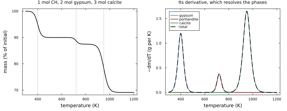
Recovering the windows from the curve
Here is why the operator is written as a smooth function of its windows. Given a thermogram, the windows are identifiable, and the machinery that says whether a parameter is determined is the machinery that determines it.
target = tg.dtg       # the model's own curve: a self-test, not a measurement

forward(θ) = thermogram(
    state, with_window_parameters(windows, θ; kind = PROV_UNSTATED);
    temperatures = grid,
).dtg

# Gauss-Newton in log space, on the same sensitivity matrix `identifiability`
# uses — the machinery that says whether a parameter is determined is the
# machinery that determines it.
function identify(θ0; iterations = 40)
    θ = copy(θ0)
    for _ in 1:iterations
        J = log_sensitivity(forward, θ)
        θ = θ .* exp.(clamp.(-(J \ (forward(θ) .- target)), -0.3, 0.3))
    end
    return θ
end

θ0 = window_parameters(windows)[1] .* [1.1, 1.4, 0.945, 0.6, 1.042, 1.4]
θ = identify(θ0)
truth = window_parameters(windows)[1]
@printf("started %4.0f K and %2.0f%% away; recovered to %.2e relative\n",
        maximum(abs.(θ0 .- truth)), 40, maximum(abs.(θ .- truth) ./ truth))
started 40 K and 40% away; recovered to 0.00e+00 relativeAnd then the question that matters more than the numbers:
id = identifiability(forward, θ; observed = target,
                     names = window_parameters(windows)[2])
id
Identifiability of 6 parameters
singular values [0.181, 0.0641, 0.0403, 0.00691, 0.00436, 0.00122]
condition 148.7
constrained 6 of 6 directions
residual RMSE 0.0
noise level σ 7.146e-12
most collinear w(Portlandite) / w(Cal) r = -0.001Six parameters, six directions constrained — because the three peaks are well separated and the curve is fitted exactly, so that the noise level takes its floor, √eps times the root-mean-square of the curve, and the standard error of every direction is far below one. That is not the usual case. The spectrum does fall by a factor of 5.8 between its third and fourth values: a log-sensitivity carries the size of its parameter, some hundreds of kelvin for a midpoint and some tens for a width. Read off that gap alone, without a noise level, the rank would have been three.
Where it stops, and why that is the useful part
overlapped = [placeholder("Gp", 400.0, 15.0), placeholder("Portlandite", 405.0, 15.0)]
fwd2(θ) = thermogram(state, with_window_parameters(overlapped, θ; kind = PROV_UNSTATED);
                     temperatures = grid).dtg
θ2, names2 = window_parameters(overlapped)
identifiability(fwd2, θ2; names = names2)
Identifiability of 4 parameters
singular values [0.0659, 0.00621, 0.000718, 0.000188]
condition 350.9
constrained 1 of 4 directions, by the gap (no noise level)
most collinear T½(Gp) / T½(Portlandite) r = -0.995p_o = plot(; xlims = (300, 520), xlabel = "temperature (K)", ylabel = "−dm/dT (g per K)", legend = :topright,
size = (720, 360), left_margin = 6Plots.mm, bottom_margin = 6Plots.mm,
title = "Gypsum at 400 K and portlandite at 405 K, both 15 K wide")
for (w, lab, c) in zip(overlapped, ("gypsum", "portlandite"), (:steelblue, :firebrick))
plot!(p_o, grid, 1000 .* thermogram(state, [w]; temperatures = grid).dtg; lw = 2, color = c, label = lab)
end
plot!(p_o, grid, 1000 .* fwd2(θ2); lw = 2, ls = :dash, color = :black, label = "what the curve shows")
p_o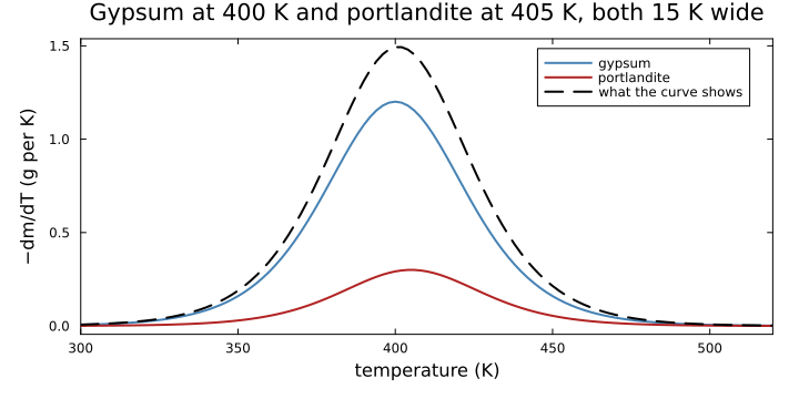
Two phases releasing 5 K apart, and the rank comes out at one of four: the position of what the curve shows as one peak, the spectrum falling by 10.6 after its first value and by 8.7 after its second. The two midpoints are correlated at −0.995, so that position is a combination of both, and two peaks with four parameters between them are not there to be seen. A fit would still return four numbers.
This is the ordinary case in a cement paste — C-S-H, AFt and AFm all release below 200 °C — which is why running identifiability on the windows is not a formality.
null_participation(identifiability(fwd2, θ2; names = names2))4-element Vector{Float64}:
0.056358824666536474
0.9999989077571443
0.9436599372207309
0.9999823303555877That is what as_traced reads to decide which parameters to report as fitted and which as PROV_PLACEHOLDER — a number the curve did not determine is one the optimizer had to leave somewhere. It reads the subspace, not the parameter's position relative to the rank: the rank counts directions, the position is the packing order, and confusing them flags whichever of a trading-off pair happened to be listed second.
What a thermogram is plotted against, and windows given as intervals
A thermobalance records the mass of the sample as it is heated (Lever et al., 2014). What the cement literature reports is the mass lost, in percent of a reference mass, and the papers co-authored by Lothenbach, whose method is set out in Lothenbach et al. (2016), do not all take the same reference. Three are in use, and the data files of this package carry each with its source:
| reference mass | used by | relative_to |
|---|---|---|
| the sample at the start of the run | the thermograms of Deschner et al. (2012) | :initial (default) |
| the dry sample at a temperature | 500 °C, (Schöler et al., 2015); 800 °C, (Shi et al., 2016) | that temperature |
| the sample ignited at 980 °C | Shi and Lothenbach (2020) | 980 + 273.15, or :ignited |
thermogram returns the mass and the loss in kilograms, and both again in percent of the reference relative_to names (mass_percent, loss_percent, the loss counted from the first temperature of the grid). The reference mass is computed at its own temperature, not read off the nearest point of the grid.
dry = literature_value("Scholer2015", "tga_dry_solids_temperature")   # 500 °C
for (label, ref) in ((":initial", :initial), ("dry at 500 °C", dry), (":ignited", :ignited))
    t = thermogram(state, windows; temperatures = grid, relative_to = ref)
    @printf("%-14s reference %7.3f g   loss at the end %6.2f %%\n",
            label, ustrip(uconvert(us"g", t.reference_mass * us"kg")), t.loss_percent[end])
end
:initial reference 718.586 g loss at the end 30.90 %
dry at 500 °C reference 628.796 g loss at the end 35.31 %
:ignited reference 496.576 g loss at the end 44.71 %fig = plot(; xlabel = "temperature (K)", ylabel = "mass lost (% of the reference)", legend = :topleft,
size = (720, 380), left_margin = 6Plots.mm, bottom_margin = 6Plots.mm,
title = "One curve, three reference masses")
for (label, ref) in ((":initial", :initial), ("dry at 500 °C", dry), (":ignited", :ignited))
plot!(fig, grid, thermogram(state, windows; temperatures = grid, relative_to = ref).loss_percent; lw = 2, label)
end
fig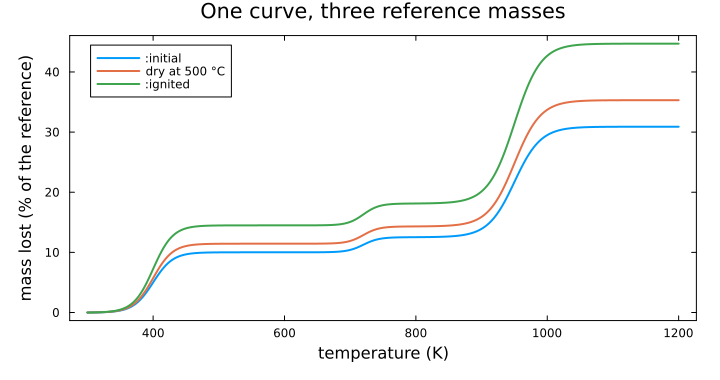
The same loss is a larger percentage of a smaller reference: which convention a measured curve follows has to be read in its paper before it is compared with one computed here.
The papers also attribute a loss to a phase by a temperature interval: portlandite between 350 and 500 °C (De Weerdt et al., 2011), the carbonate from about 300 to 850 °C (Shi et al., 2016), the water of ettringite between 30 and 150 °C (Möschner et al., 2009), the total bound water between 30 and 550 °C (L'Hôpital et al., 2016). A window can be given that way, between = (T₁, T₂): the phase then releases everything inside the interval and nothing outside it, along a smooth step whose rate vanishes at both ends. literature_windows gives such a window for every release of a state at once, from these four papers: the water of portlandite and of the ettringites over their own intervals, that of every other hydrate over the interval of the total bound water, the carbon dioxide over that of the carbonate.
ch = literature_table("DeWeerdt2011", "tga_intervals")
cc = literature_table("Shi2016", "tga_intervals")
from_papers = [
    windows[1],      # gypsum: no interval in these papers, the placeholder kept
    DecompositionWindow("Portlandite"; between = (only(ch.lower), only(ch.upper)),
                        kind = PROV_PUBLISHED, source = "DeWeerdt2011"),
    DecompositionWindow("Cal"; between = (only(cc.lower), only(cc.upper)),
                        releases = :carbon_dioxide, kind = PROV_PUBLISHED, source = "Shi2016"),
]
T1, T2 = window_interval(from_papers[2])
t = thermogram(state, from_papers; temperatures = [T1, T2], relative_to = dry)
inside(phase) = t.by_phase[phase][2] - t.by_phase[phase][1]
@printf("lost between %.0f and %.0f °C: %.3f g of portlandite water, %.3f g of calcite CO2\n",
        T1 - 273.15, T2 - 273.15, 1000 * inside("Portlandite"), 1000 * inside("Cal"))
@printf("portlandite holds %.3f g of water\n",
        ustrip(uconvert(us"g", Dict(bound_water_per_phase(state))["Portlandite"])))
lost between 350 and 500 °C: 18.015 g of portlandite water, 36.603 g of calcite CO2
portlandite holds 18.015 g of waterThe interval gives the portlandite all its water and nothing else. The loss read over that interval holds more: the carbonate's interval overlaps it, and part of the calcite's carbon dioxide leaves between 350 and 500 °C as well, which is the loss a reading has to separate (L'Hôpital et al. (2016) quantify portlandite from the loss around 450 °C by the tangent method). A logistic window spread over the same interval, 1 % released at one end and 99 % at the other (window_interval), would put 2 % of the portlandite's water outside it. Both forms can be mixed in one set, fitted to a curve (window_parameters gives an interval's two ends), and read by bound_water over a temperature range, as a recipe's bound water is compared with a measurement.
See also
CEM I 52.5 N and slag in an isothermal calorimeter, read off the states, the heat of the same pastes.
The water budget of a hydrating paste, what bound water is and why the pore solution is not it.
Where the numbers come from, provenance and what to do when the number does not exist yet.
Calibrating hydration kinetics, where the correlations calorimetry leaves call for a second measurement.